Introducción

Prediction and forecasting have been a topic of great interest in the data mining community. Most of the work in the literature has dealt with discrete objects such as: keystrokes, database queries, medical interventions and web clicks (¹⁹, ³²). However, prediction may also have great utility in real-valued time series. We briefly consider two clear examples. The first one fits in the robotic interaction field, where researches noted the importance of enabling robots with a short-term predictive capacity, to control the impedance forces generated by its interaction with humans (¹⁰). Secondly, mining real time weather data to discover predictive rules. The Doppler radar technology introduced in the last two decades, has increased the mean lead time for tornado warnings from 5.3 to 9.5 minutes. But progress seems to have stalled. Around 26% of tornados within the US occurs without warning (³). McGovern et al in (³), argued that further improvements will come not only from new sensors, but also from yet-to-be-invented algorithms that can examine existing data to discover predictive rules.

Most of the current work has attempted to predict the future based on the current value of a stream (²¹). The actual values are, in fact, nearly irrelevant, but the shape of the current pattern may generate better predictive rules.

There is a critical distinction between forecasting and rule-based prediction. The forecasting approach is typically always-on, it predicts values at every time step. In contrast, “rule-based” predictions monitor the incoming data at each time step, but only occasionally, makes a prediction about an imminent occurrence of a pattern. On this line, Mohammad Shokoohi-Yekta et al in (²⁸), proposed a rule discovery framework to identify patterns in time series. All these discovered rules, are generated from a ranked candidate list of motifs: a subsequence of the time series is identified twice or more. The motif classification algorithm is computed using Euclidean distance, a widely-known similarity measure

(⁷). The present work makes four main contributions. First, we upgraded the rule discovery framework created by Mohammad Shokoohi-Yekta et al (²⁸), by incorporating three well-known similarity measures: 1- Manhattan, 2- Minkowski and 3- Dynamic Time Warping.

Second, we added an enhanced and novel version of Dynamic Time Warping (DTW), proposed by the authors in (¹⁴), which uses a Cubic Spline Interpolation technique that is capable to produce much less singularities and obtain the best warping path; especially when time series are not suitable for the standard DTW.

Third, we utilized the upgraded version of the framework to carry out a benchmarking for all the these similarity measures. This effort intended to proof that DTW based on Cubic Spline Interpolation (SIDTW), can be as efficient as the Euclidean distance to discover meaningful rules in time series.

Finally, we developed a new functional layer upon the framework, to automate the discovery and testing of rules from time series, given a particular similarity distance.

The remainder of the paper is structured as follows. Section two introduces the related work and the intuition behind this shape-based mechanism to identify potential rules in time series. The rule discovery framework is detailed in section three. The experiments have been developed to characterized each similarity measure running upon this framework, its results are discussed in section four. Finally, the conclusions of this research and its speculation about the future work are proposed in section five.

Background

In a set of papers ending in (²⁵), Park and Chu suggested a rule finding mechanism for time series. Their algorithm was evaluated for speed, using random walk data. No evidence was reported that the algorithm could actually find generalizable rules in time series. The research done by Wu and colleagues in (³³), did use a piecewise linear representation to support rule discovery in time series. They tested their algorithm on real (financial) data, reporting roughly 68% “correctness of trend prediction”. The authors ran their algorithm on data provided by others. When they ran their program using pure random walk data, they claimed to get again about same 68% correctness of trend prediction. The latter suggests that their original results did not outperform random guessing.

Probably of the most cited rule finding method found in the literature is (⁶). This research quantizes the data with K-means clustering. The whole training dataset passes data over to the typical association rule discovery algorithm. A further set of corrective articles showed that there is an evident problem with the quantization step. In summary, any method that involves clustering the whole set of subsequences, is mis-driven to produce cluster centers that are independent of the data (¹⁶).

The work of Mohammad Shokoohi-Yekta et al, cited in (²⁸), is the backbone of this research. They created a framework to discover and test rules on time series. The solution was designed to identify potential rules known as subsequence motifs (discoverRules()). A classification algorithm powered by Euclidean distance, produces predictive rules (testRules()) from all the motifs identified.

While there are a vast list of distance measures in the literature, recent empirical evidence suggests that Euclidean distance is very difficult to beat (⁷). The Euclidean distance is simple to implement, parameter free, fast to compute and also amiable to various data mining optimizations, such as indexing and early abandoning computation (²³).

The authors in (²⁸) also considered other distance measures such as: DTW, Swale, Spade and EPR (⁷). They empirically claimed that none of these similarity measures actually helped to improve the accuracy, and even worse, most of them required a runtime at least an order of magnitude longer.

In (³⁵) the authors introduce an approximate algorithm called HierarchIcal based Motif Enumeration (HIME) to detect variable-length motifs with a large enumeration range in millionscale time series. The authors show in the experiments that the scalability of the proposed algorithm is significantly better than that of the state-of-the- art algorithm. Moreover, the motif length range detected by HIME is considerably larger than previous sequence-matching based approximate variable-length motif discovery approach. They demonstrate that HIME can efficiently detect meaningful variable-length motifs in long, real world time series.

In this project, we study the accuracy obtained by different similarity measures, particularly through the implementation of DTW and SIDTW (²⁷, ¹⁴).

The details about the rule discovery framework are presented in the following section.

Rule discovery framework

We are now in a position to develop all the required concepts to explain the rule discovery framework. First, we define a time series “antecedent” as a subsequence is triggered only if it is similar to the current sliding window.

In order for a candidate antecedent to be even considered as a rule precursor, it must occurs at least twice. We cannot generalize from a single instance of an event. This is the most basic definition of a time series motif (²²).

As an antecedent is a precursor to an event, a predicted subsequence shape, which follows an antecedent within a specified time (the maxlag), is called the antecedent’s consequent.

The maxlag parameter encodes the fact that for a time series subsequence to be a meaningful consequent in a rule, it must occur within some acceptable time, after the rule’s antecedent has been detected. Without such a constraint on time, a consequent’s occurrence may be a mere coincidence.

In principle, the threshold, the maxlag and antecedent could be hand chosen by a domain expert.

All the concepts described above can be formally summarized in 5 simple definitions:

Having defined time series rules and the supporting notation, we can describe the mechanism behind the rule discovery task.

The Required Intuition Behind The Rule Discovery Process

A simple application example explains the basic cognitive process towards the discovery of meaningful rules in time series. We utilized an accelerometer to collect data from a device worn by a person, as he or she goes about daily activities. Let’s say, for instance, walk and use an elevator, as it is shown in Figure 1.

Figure 1 A rule found from an accelerometer dataset by using an elevator. 

A rule for an accelerometer dataset identifies the initial acceleration “bump” as going up in an elevator. Which must be eventually matched by the elevator stopping at a floor. This example shows a very easy rule to spot. The semicircular bump (antecedent subsequence - red highlighted) created by an elevator accelerating, must eventually be matched up, by a bump in the opposite direction (consequent subsequence - green highlighted) when the elevator brakes. The time lag (maxLag, set to 4 seconds) between these two events is highly variable. It depends on the number of floors serviced by the elevator.

The Rule Discovery Framework

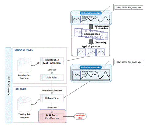
Once the above concepts have been defined, the rule discovery framework can be logically divided into two main basic modules. The first one, called “Discover Rules”, was created to search rules from a given input training set, a split point value and a maxLag value. As it is shown in figure 2, the first section of the algorithm will invoke a discretization process, to extract all the potential rules (motifs). The evaluated subsequences are divided into antecedent and consequent (using a split-point). The algorithm will slide each antecedent subsequence across the entire data set, searching for a similar shape, identified at least twice. This motif identification process is obtained as a result of a similarity computation between both subsequences: 1- a subset of the training set and 2- the antecedent subsequence that is being compared (²⁸).

Figure 2 Diagram of the framework designed to discover and test rules. 

The second module, called “Test Rules”, also detailed in figure 2, was created to score and classify any antecedent subsequence extracted from the “Discover Rules” module.

The scoring algorithm uses minimum description length (MDL). It uses two inputs parameters: 1- a candidate time series and 2- an expected maxlag value. The function then returns three objects: an antecedent, a consequent and the “quality” score value of the resulting rule (²⁸). In the subroutine, we use a similarity distance measure to create a large set of candidate rules with their observed outcomes on the training data. We move from Euclidean distance to MDL to score these rules.

We consider the consequent of R, as a model (a set of hypothesis) to calculate the total number of bit-saves to predict other consequents segments. A larger number of bit-saves indicates more accurate predictions. After discovering antecedent candidates, we consider their following subsequences as consequents. The procedure calculates the number of bits needed to record the differences between the consequent saved as a model and the subsequences following antecedent candidates (²⁸).

Finally, the number of firings depends on the distance threshold chosen. A conservative (small) threshold is more likely to produce an accurate rule, but, it may miss opportunities when it could have fired and produce predictions that are at least much more better than random (²⁸). The motifs that fire the most during the testing process are the ones suggested as a meaningful rule.

Our Contribution To The Framework

There are four major contributions in this work. First, we endowed the existing framework with three well-known similarity distances: Manhattan, Minkowski, Dynamic Time Warping (DTW). Second, we added an enhanced and novel version of DTW called SIDTW, which was proposed by the authors in (¹⁴). Third, we ran a benchmarking analysis to study the accuracy produced by all of these similarity distances. Finally, we developed an automated way to discover and test rules from time series, given a particular similarity distance.

The framework was initially implemented by using the Euclidean distance (⁷). Given two time series Q and C of length n, where Q = q ₁ , q ₂ , q ₃ , q _i ...q _n and C = c ₁ , c ₂ , c ₃ , c _i ...c _n , the Euclidean distance is defined as As was mentioned, the framework was also equipped with two Lp shaped-based distances, the Manhattan distance (⁷), defined as: . The Minkowski distance, formally implemented as , where p is an integer threshold.

In addition to the previous L p shaped-based distances, we implemented an elastic-based version of DTW (²⁷). This efficient implementation of DTW was written in C language. This standard version of DTW taken from (²⁷), can be formally defined as where W is the minimum path.

As it is known, this distance finds an optimal match between two sequences of feature vectors, which allows for stretched and compressed sections of the sequence (²⁷).

Why SIDTW was proposed in this project?

Dynamic time warping (DTW) and derivative dynamic time warping (DDTW) are two robust distance measures for time series. The algorithm allows similar shapes to match even if they are out of phase in the time axis (²⁷).

We added a new version of DTW based on cubic spline interpolation (SIDTW) (¹⁴), mainly based the educated assumption that its the level of accuracy was way superior than the other distance measures.

How does it work? The derivative of every point of the time series is computed by cubic spline interpolation. This method is utilized to replace the estimated derivatives in DDTW. After interpolation, SIDTW uses derivative-based sequences to represent the original time series, which is way better to describe the trend of the original time series and more reasonable to warp (¹⁴). The authors in (¹⁴), empirically indicate that the quality of similarity measure, for the three warping methods, is nothing to do with the amount of warping (¹⁴). They experimentally perform the proposed method and compared with the existing ones, which demonstrates that in most cases their approach not only can produce much less singularities and obtain the best warping path with shorter length but also, is an alternative version of DTW when time series datasets are not suitable for DTW to be measured.

There is an index W proposed in (¹⁴) to indicate the warping level implied in the algorithm. For instance: where K is the number of warping and m is the length of time series. In this formula, it is clear that W is in direct proportion to K due to the constant length m. In addition to that, the small W is, the less amount of warping will be produced. The DTW algorithm will run prior any cubit spline interpolation activity. That should happens in order to avoid unnecessary warping.

The SIDTW algorithm can be presented as follows:

There are at least three main benefits in SIDTW: 1- the points with positive derivative in one sequence will align each other on the same trend, 2- in most cases, the length of the warping path will be shorter than the DDTW and DTW, including a less number of singularities as was already mentioned and 3- SIDTW is an alternative version of DTW. Therefore, the SIDTW measure the similarity of most of time series datasets but in any other case, DTW can be also use instead.

The experimental evaluation of all these distance measures is presented in the next section.

Experiments

In this section we evaluate the performance of each similarity measure that was ran to discover and test rules in time series in the upgraded framework. We compared both algorithms (discoveryRules and testRules). That allowed us to determine which similarity measures were generating the best possible results on each data set.

All of our experiments have ran on an Intel64 processor with approximately 2295 MHz, upon MS Windows 8.1 OS. In order to reproduce these experiments, the following software is required: IDE: Matrix Laboratory (MATLAB), version 9.1.0.44, 64-bit, IDE: RStudio, version 1.0.136, 64-bit, Libraries: PMCMR, nortest, TSdist version 3.3, proxy version 0.4-17, sampenc and RunRcode.

About the data sets that were utilized in this project

We did use the seven different datasets provided in (²⁸). There are two specific reasons for making that decision. The first one, is mainly to proof the veracity of their results, using the Euclidean distance as a reference. The second and most important reason, was lead by the consistency and the simplicity of studying the behavior of new distance measures against the same datasets.

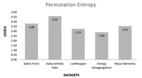
A new dataset was generated to increase the impartiality level of the experiment. To achieve the latter, we use a time series generator described in (¹²). The tool captures daily activity data in a time series format. This new dataset offer a new level of complexity, which can be defined by two different characteristics: 1- is the dataset with the smallest amount of data points and 2- it contains the highest degree of data level disorder or noise. The permutation entropy obtained from this dataset is observed in Figure 3. This metric was very useful to measure the degree of disorder found on each time series (³¹).

Figure 3 Permutation entropy levels computed on each dataset. 

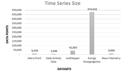
An impartial sample of experimental datasets, should consider a variation in the number of data points of each dataset and different levels of disorder and permutation entropy. This combination of factors are imperatively required to categorize the complexity of each dataset and then quality of the experiment. (³¹). The Figure 4, describes for instance, the number of data points on each dataset in this experiment. (³¹).

Figure 4 The number of data points on each dataset. 

We are in a position to present the results that were obtained from each distance measure on every single dataset. In the more general case, we use a given distance between the predicted consequent and the F matching locations where the rule fired, a value we denote as F _error (this is essentially the root-mean-squared error). Because this number is difficult to interpret by itself, we do the following: on the same testing set, using the same consequent, we fire the rule randomly, F times, and measure the distant between the predicted consequent and the F random locations. We denote this value as R _error (which is averaged over 1.000 random runs).

The reported measure of quality then is just (Q = F _error /R _error ). Values close to one suggest the rules are no better than random guessing and values significantly less than one indicate that there is a true structure in the data.

The hypothesis Q is defined as the accuracy reported by the distance measure to find a meaningful rule in a particular dataset. Again, the size and the complexity of each dataset are considered relevant factors to achieve the expected quality in this experiment. Our hypothesis was tested by using the nonparametric test called Kruskal-Wallis (³⁴). The assumptions of oneway ANOVA were not met (p-value = 0.4409, using a = 0.05). Due to the obtained results, we do believe that there is no strong statistical evidence to categorically support our hypothesis. The margins of these results are not significant.

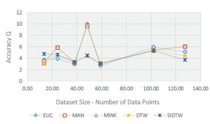
Despite the above given outcome, we want to highlight some interesting observations. In the Figure 5, the SIDTW distance measure did report higher accuracy levels (where Q average values close to zero, suggest a higher accuracy level), particularly when the number of data points on each dataset tended to increase. For instance, SIDTW has reported better results than the Euclidean distance, including the standard version of DTW.

Figure 5 Accuracy per distance measure. 

The SIDTW did report also better results in presence of highest degrees of permutation entropy. As was shown in the Figure 6, this novel similarity measure, was even more tolerant than the Euclidean distance, to deal with higher entropy levels and report out, at the same time, the best average values of Q on each dataset.

We ran the testRules() algorithm (based on the values obtained from discoverRules()), using all the distance measures on each dataset. As was mentioned, every distance measure was executed 1000 times on each dataset for this algorithm as well, in order to control the factors of the experiment and its consistency. Finally, we did a simple data normalization process (without losing precision), in order to get the average value of Q, for each combination of factors.

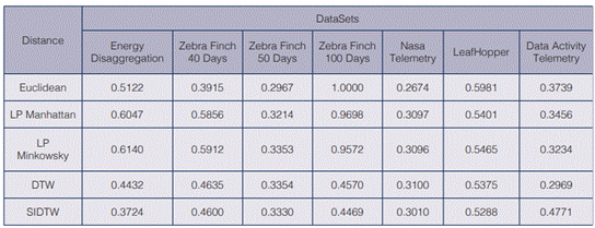
In Table 1, we present the average values of Q, for every factor. The green highlighted Q figures, on every row, represent the best results of a given similarity measure executed on each dataset. The red highlighted figure correspond to the worst possible value. As the Euclidean distance, SIDTW did report the best results of Q in three times. DTW in general, shows to be a reliable distance measure. At least as good as the Euclidean distance.

Table 1 Average result of Q, per every combination of factors resulted from the testRules() algorithm. 

Conclusions and future work

We have presented an upgraded version of a framework created in (²⁸). The tool discovers meaningful rules in time series using SIDTW. The major contribution of this research is the implementation of four new similarity measures: L _p Norm Manhattan, L _p Norm Minkowski, DTW and DTW based on Cubic Spline Interpolation (SIDTW). A brand new dataset was generated from the scratch to support the veracity of the experiments reported by the authors in (²⁸) and increase the quality of our experiments. The experiments have been uploaded at (¹¹). The automated testing of motifs was integrated as a new module.

We ran a hypothesis testing to study the accuracy levels (Q), obtained from the utilization of SIDTW, as a novel distance measure proposed in (¹⁴). This analysis showed that SIDTW is as good as the widely implemented Euclidean distance.

Finally, many other avenues can boots this research initiative to the next level. For example, exploring the insertion of new types of similarity distances, such as: elastic, lock-step and threshold-based (⁷). Further metrics can be added: execution time, precision levels and efficiency. We considered to increase the scope of the framework adding others data mining duties such as outliers detection and clustering.

Acknowledgment

In the first place, we thank Mohammad Shokoohi-Yekta et al, for providing us with a welldocumented, debugged and available on-line version of the framework written in MatLab.

We also thank to Cindy Calderón Arce, from the Instituto Tecnológico de Costa Rica, for her valuable help, to guide us in the right track of knowledge and references, to resolve the challenge of dealing with time series with different lengths; a fundamental data preparation activity, required before applying any similarity computation.

Finally, the authors would like to thank the Maestría en Computación program at Instituto Tecnológico de Costa Rica for providing the occasion for this research.