


 Spanish (pdf)
 Article in xml format
 Article references
 Send this article by e-mail
 Cited by SciELO
  Similars in
SciELO
Similars in
SciELO 
 Permalink
Introduction and State-of-the-art
Although the incidence of gastric cancer has been decreasing, it is still the 5th most common and 7th most prevalent cancer worldwide (Bray et al., 2018).
Through the mid-nineties, it was the primary cause of cancer-associated death worldwide, and, in the most recent years, it has been the 3rd most deadly, causing approximately 783,000 deaths per year (Rawla & Barsouk, 2019). Because Helicobacter pylori is an important agent in developing gastric cancer in humans (Rawla & Barsouk, 2019), there is an interest in the study of this bacterium. Infections from this bacterium induce proliferation of gastric epithelial cells with a risk of evolving into metaplasia, dysplasia, and invasive gastric cancer (Correa & Houghton, 2007). Pathologists use immunohistochemistry for diagnostics, which consists in the use of antibodies to identify antigens (also called markers) inside a tissue sample (Duraiyan et al., 2012). One of these markers is called Ki-67, and it is highly associated with the proliferation of cells (Li et al., 2014). Cells containing the antigen are stained, which allows them to quantify Ki-67 positive cells in the sample.
Quantifying the Ki-67 stained cells can be conducted using open-source programs and commercial software. These applications automate the process to some extent. For example, in the case of QuPath (QuPath, 2021), it is necessary to follow some steps: annotate the regions of interest (ROI); run the cell detection command indicating parameters such as type of tissue, pixel size, maximum and minimum nuclei area; train a classifier based on the annotations; finally, obtain the positive and negative cell count. On the other hand, ImageJ has a plugin called ImmunoRatio (Tuominen et al., 2010), which calculates the Ki67 index based on nuclei area ratio. In this case, it is also necessary for the user to indicate a series of parameters, for example, the segmentation thresholds for the nuclei (Yeo et al., 2017). Other methods have been developed using techniques like k-means clustering for breast cancer histology images (Al-Lahham et al., 2012) or for human nasopharyngeal carcinoma xenografts images (Shi et al., 2016). In Barricelli et al. (2019), Bayesian classification trees are used, and in Xing et. al. (2014), the seed of the cells is located in order to classify them based on geometric descriptors, color intensity, cell morphology, and histogram intensities. However, these methods work for images whose staining is well marked, for example, with brown and light blue. There are also commercial programs such as the Aperio IHC Nuclear Image Analysis Tool (Aperio, 2007), which provides the option to annotate ROI and the complete automation of the whole quantification process. The problem with commercial programs is that they are neither free nor open source, reducing accessibility and customizability.
In the case of H.pylori-induced proliferation, immune cells infiltrate the gastric epithelium and start proliferating as part of the immune response to the pathogen. However, in many cases, pathologists are interested in the proliferation of epithelial cells and disregard these proliferating immune cells according to their location within the tissue. With the methods explained before, pathologists would be required to review and fix the automatic results by conducting the analysis, which negates the advantages of automation. Importantly, Ki-67 staining is used to measure proliferation in other tissues; therefore, a tool that can accurately quantify proliferation and can be customized to different tissue structures is of great value. This work presents an automated Ki-67 quantification algorithm. It works for image sets with lower contrast in the staining and only requires the user to delimit the ROI (with an image analysis tool) where the quantification should take place (correctly marking the ROI by an expert can influence the accuracy of quantification).
Methodology
Modeling the Intensity of the Nuclei’s Pixels
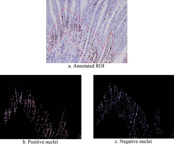
The ROI of the images in the dataset were manually annotated by an expert with QuPath and a red border line, as shown in Figure 2a, in order to delimit the processing to only the relevant part of the images. Afterward, a representative proportion of both Ki-67 positive and negative cells within the ROI of 10 images were manually annotated (labeled as images 1 to 10), for a total of 5702 Ki-67 positive and 6248 Ki-67 negative cells, see Table 1 (the ground truth data is available on request). For images 6 to 10, the manual counting of all the nuclei inside the ROI was performed, and the manual Ki-67 index was obtained. The first five images were only used to obtain samples of the color distributions of the nuclei but were not fully annotated. The annotations were done with an elliptical shape border, which allowed approximating the actual nuclei shape. Each ellipse is described by its center (m,n) and the lengths of its horizontal and vertical axes, a and b, respectively. These ellipses were used to draw binary masks with OpenCV that will be used to select pixels' samples to build a model for the classification. In order to remove any pixel not related to the specific type of nuclei, a bitwise-AND operation was carried out between the selected images in BGR and the masks generated before. The distribution of the pixel intensity of each nuclei type was analyzed via its histogram.
The resulting masked BGR image was converted to HSV and grayscale for the positive and negative nuclei, respectively. In the case of the positive nuclei, the V channel was used. Usually, the Ki-67 staining has good contrast between the color (brown) and the counter-color (light blue); so, at first, the H channel was the main candidate. However, in some of the images of the dataset, the counter-color, instead of being light blue, appeared to have a shade of purple and pink, while the color of the Ki-67 appeared to have a shade of auburn and purple. This was then reflected as low contrast in channel H images. On the other hand, the variation between color and counter-color was based to a greater extent on the darkness of the purple-brown tone, so the V channel was a better choice. Concerning the negative nuclei, the V channel was not so useful because it showed low contrast between the background and negative nuclei. Therefore, the grayscale was chosen.
Table 1 Manual Count of Ki-67 positive and Ki-67 negative nuclei.
| Image/Ki-67 | 1 | 2 | 3 | 4 | 5 | 6 | 7 | 8 | 9 | 10 | Total |
|---|---|---|---|---|---|---|---|---|---|---|---|
| Positive | 231 | 261 | 261 | 297 | 166 | 629 | 434 | 1220 | 1001 | 1202 | 5702 |
| Negative | 133 | 172 | 192 | 156 | 185 | 731 | 866 | 1563 | 1119 | 1131 | 6248 |
| Total | 364 | 433 | 453 | 453 | 351 | 1360 | 1300 | 2783 | 2120 | 2333 | 11950 |
Note: derived from research.
Based on the histograms of the cells, for both the V channel and grayscale, Gaussian models were chosen to represent each distribution of the pixels X ∼ N (x̄ , s2). The mean and standard deviation were calculated as in equation 1. In this equation, L is the amount of pixel intensities, hi is the value for the given histogram bin, and i represents the bin number.

The images with Ki-67 staining tend to have two types of quality problems: the uneven gathering of pigment on stained tis-sues and small pigment particles scattering around (Shi et al., 2016). Because of this, the first step was to apply a Gaussian blur filter to the original BGR image in order to eliminate noise and smooth out the image. After filtering the image, it was converted from BGR to HSV, and the V channel was then segmented via thresholding. The seg-mentation was carried out as in equation 2, where T1 and T2 are the thresholds, α is a parameter that determines the number of standard deviations to consider, and f and g are the original and segmented images, respectively. This resulted in a mask for all the positive nuclei, and, finally, this mask was applied to the original BGR image to obtain the segmented Ki-67 positive nuclei.

Like Ki-67 positive nuclei, for the Ki67 negative nuclei, the first step was to apply a Gaussian blur filter to eliminate noise and smooth the image; the difference is that, for the negative nuclei, the grayscale image was chosen. The segmentation was also carried out as in equation 2, which resulted in a mask that was applied to the BGR origina image to obtain the segmented negative nu-clei. However, this last image had residues of the Ki-67 stain pigment around the re-moved positive nuclei. This was removed by carrying out a bitwise-AND operation with the positive nuclei mask, but before this operation, the mask was dilated in order to cover more of the residues. Finally, an opening operation was applied to the image to remove any last particles.
Calculating the KI-67 Index
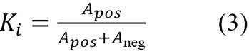
The nuclei in the training images have variations in morphology. Some have a shape like a circle, some to an ellipse, and some have a shape that cannot be so easily associated with a regular figure. Also, some nuclei are bigger than others and have different orientations. Because of this, we decided to calculate the Ki-67 index (Ki, see equation 3) as the ratio of the area of the segmented positive nuclei (Apos) to the area of all the segmented nuclei (Apos + Aneg), as studied in Barricelli et al. (2019), instead of counting each nucleus individually:
Analysis and Results
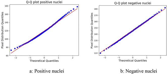
The parameters of the Gaussian model for the nuclei segmentation were calculated. For positive nuclei, the V channel mean was 121.341; the standard deviation, 23.898; and the α parameter, 1.6. For the negative nuclei, the grayscale mean was 145.506; the standard deviation, 15.600; and the α parameter, 1. The Q-Q plots in Figure 1 were used to determine whether the model selection introduced a substantial error. As can be observed, most of the points lie on the 45º line. The dotted curve seems to deviate downwards, which indicates a slight skew to the right. The root-mean-square error (RMSE) for this fit is 0.440 for the positive nuclei and 0.430 for the negative nuclei. In a perfect Gaussian distribution, the mean and the median coincide; therefore, in order to quantify the amount of error the skew brings into the model, the difference between these metrics was calculated. The average difference for the positive nuclei was 1.45%, and for the negative nuclei, 0.45%.
Figure 1 shows the results of segmenting the positive and negative nuclei. As shown in subfigures 2a, 2b, and 2c, the automated quantifier segments only the nuclei inside the ROI.
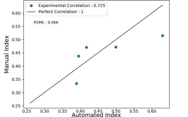
Table 2 summarizes the Ki-67 indexes obtained for each validation image both by the algorithm and manual counting. The smallest error between indexes was 5.720%, while the highest was 22.330%, giving an average error of 13.159%. Figure 3 shows the correlation between the automated and manual Ki-67 index, which resulted in a Pearson correlation of 0.725, with an RMSE of 0.066.
Discussion and Conclusions
This study developed an automated approach to estimate the Ki-67-index that does not require prior experience with cell counting and accepts images with annotated ROI. As shown in Figure 2, the proposed method can segment both the positive and negative nuclei that reside in the previously annotated ROI. Based on the area of the segmented nuclei, the automated method calculates the Ki-67 index with a strong Pearson correlation of 0.725 when compared to the manual method. This gives certainty that the automated method can be used to analyze an increment of stained cells.
Note: derived from research.
Figure 1 Q-Q plot for the Gaussian model of the positive and negative nuclei.
Note: derived from research.
Figure 3 Pearson correlation between the automated and manual Ki-67 index for images 6-10.
On the other hand, the Ki-67 indexes calculated by the automated method have an average difference of 0.057, an average square difference of 0.172, and a RMSE of 0.293, compared to the manual method, as shown in Table 2. It is equally important to evaluate both the error of the automated method and the accuracy of the insight these indexes provide. The St. Gallen International Consensus of Experts (Goldhirsch et al., 2011) recommends the categorization of the Ki-67 proliferation index into 3 groups: low (Ki-67 ≤ 15%), intermediate (15% < Ki-67 ≤ 30%), and high (Ki-67 > 30%). Based on these categories, the indexes calculated by our algorithm provide the same classification as manually determined by a trained expert. There are different error sources for this method. The Q-Q plots showed that the model selection introduced minor errors. In addition, an important parameter for these Gaussian models is α because of its direct relation with the index. The value corresponding to the α parameter for the positive nuclei was determined experimentally by means of a visual inspection of the segmentation of the V channel, similarly the α parameter for the negative nuclei was experimentally determined using the grayscale image. These parameters can be optimized by using a train/test/validation split. Despite the small sample size, we demonstrated the utility of our method. However, the low number of scored images did not allow us to fully sample the ranges of pixel values and intensities observed by pathologists. In future work, we will explore the use of kernel density estimation, optimize α, consider morphological features for segmentation, generate a new set of synthetic images, and subsequently access a larger dataset.
Acknowledgments
We thank Alexander Sheh, Ph.D., from the Division of Comparative Medicine (Massachusetts Institute of Technology), for providing the images and insight for the present work. Also, to Rafael Chacón, M.Sc. (i.f.), for the help with the editing of the paper.

