1. INTRODUCTION
The analysis of uncertainty of land value models is a critical issue for policy formulation (1). However, while the use of Gaussian simulation to understand uncertainty has long been applied to physical land variables (e.g., (2)) and despite kriging having been applied to land rents for at least 20 years (1), no previous cases of conditional Gaussian simulation applied to land value modeling were found .
In general, the analysis of land value in the San José metropolitan region (GAM) has been fragmentary (1). Recent efforts from extension and research projects at the University of Costa Rica, however, have yielded a data set of real estate listings that provided the first synoptic view of real estate prices in the region (3). Based on this data, hedonic price models of housing have been produced (3,4) and the first efforts at extrapolation of land values for the entire region (based on kriging and co-kriging) were developed (1). To isolate land values, (1) consider in their analysis only lots —i.e., properties offered in the land market with no buildings on them and, therefore, with prices only reflecting the attributes of land—; these initial efforts yielded estimates of mean values and of variance, but they were limited to the kriging and co-kriging models.
Given the current state of the question, two objectives are proposed for this paper: first, to extend previous work on land value extrapolation (by (1)) to include conditional Gaussian simulation and, specifically, to include uncertainty estimates for the predicted land value that can be derived with this method; second, to explore whether the uncertainty of these estimates can be explained by spatial structure (indeed, by the same spatial structure related to the point pattern of real estate listings and to the land value pattern itself).
2. METHODOLOGY
2.1 Land values in the GAM
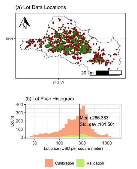
Data were compiled by (1) from real estate listings published on the web during 2020-2023. From an original data set of 3670 records with known location and price, extreme values (for the variables price, lot area, and price per square meter) were filtered out, resulting in a final data set of 3196 records. This data set was, in turn, divided by randomly selecting approximately 10 % of records: a calibration data set of 2878 records and a validation data set of 318 records result from this data wrangling process.
The final data sets (of calibration and validation) are shown in Fig. 1. Locations in panel (a) coincide mainly with the urban fabric of the GAM. It is worth noting that the calibration data seem to include a greater proportion of locations in the more central locations (or, conversely, the calibration data are distributed in a way that should better represent the peripheral land values). The land value per square meter was transformed into logarithms (as in (1), (3), (4) and, more generally, following a standard practice in the analysis of land values). The logarithmic transformation of both the calibration and validation data sets (panel (b) of Fig. 1 presents the histogram with a logarithmic scale on the horizontal axis) show a normal distribution, as should be expected, although with some degree of skew towards the left (this may be explained because the filtering process of extreme values is more efficient in excluding excessively large values of price, area, and price per unit of area).
2.2 Geostatistical analysis and conditional Gaussian simulation
As the final objective of the modeling efforts is to produce a spatially explicit prediction of land values per square meter, which is essentially an extrapolation, ordinary kriging was selected to generate a linear weighted estimation for land values at unknown locations from the data set (5), (6), (7).
In kriging, the spatial dependence structure is modeled through a semivariogram, a function that relates the mean semivariance (the squared differences in the Z value for pairs of locations xi, for locations with known Z values) for all N pairs of locations within a range of distances h (1),(6),(7):
The empirical semivariogram is fitted by a function with a specified form; for the GAM, (1) proposed a spheric adjustment; the gstat package can dete
Ordinary kriging chooses the optimal weights by minimizing kriging variance, which can be determined from the semivariogram model (5),(6).
Under the kriging method, the predicted Ẑ values for xi locations with unknown land values result from a weighted average of locations (with weights wi) with known land value, Z(xi):
Ordinary kriging chooses the optimal weights by minimizing kriging variance, which can be determined from the semivariogram model (5),(6).
The uncertainty estimate for the extrapolation was determined using sequential Gaussian simulation, which is a technique to systematically simulate realizations of a random field. Given a semivariogram from the data and a random path through all locations with no known values (such that each location is only visited once), the sequential Gaussian simulation algorithm proceeds as follows: (1) it searches for all sampled data and for all previously simulated locations, (2) it applies kriging to neighboring points and determines from it the linear estimate and its variance, (3) sample the value from a normal distribution with mean and variance from the kriging of the previous step, (4) assign the sampled value to the location and proceed along the random path to the next location (5). The simulation is termed conditional because it is conditioned on the data, via the kriging.
One hundred instances of land value patterns were simulated using conditional Gaussian simulation; at each instance, only the closest 320 points to the location being extrapolated (approximately 10 % of the calibration data) were considered in the kriging. Data on each simulated instance were back-transformed into their original units. Based on these simulations, the following metrics were reported: (1) the E-Type prediction, which is the per location (i.e., ensemble) mean of the land value (5), (2) the per location standard deviation and coefficient of variation (the coefficient of variation is the ratio of standard deviation to mean), and (3) the per location 95th and 5th percentiles, as plausible bounds within which the actual land value should be found. Calculations were performed using the gstat package (8) of statistical software R (9).
2.3 The determinants of uncertainty: an exploration of social and physical factors
The pattern of the simulated standard deviations was analyzed to explore its association with other possible spatial factors, in line with the objectives proposed. The variance follows a χ2 distribution. Therefore, to find the statistical significance of the variation in the standard deviation associated to any given factor, the following approach was employed: for all locations in the prediction space, (1) histograms were computed for each spatial factor and the locations were classified into three separate groups based on limits defined by changes in the histograms of the spatial factor; (2) a Kolmogorov-Smirnov non-parametric test was conducted to determine whether the statistical distribution of the standard deviation of any group was different from each of the other groups (for each factor separately); (3) smooth kernel densities were estimated for each group (using the geom_density() function of the package ggplot (10) from R (9)); these densities were compared. The relative positioning of the different kernel densities (determined by the group) was interpreted to understand how the factor affected the standard deviation. The general expectation was that factors associated with greater suitability for urban land use such as flatter terrain and greater accessibility would present less uncertainty, as they should also be correlated with greater density of locations with known land values (11).
Following (12), the Kolmogorov-Smirnov test is the most common instrument to explore the hypothesis of whether two samples are taken from the same statistical distribution. Taking two samples, x1, …, xm and y1, …, yn from two distribution functions, F and G, one may form the empirical distribution functions Fm: =| {xi: xi ≤ x} |/m and Gn: =| {yi: yi ≤ y} |/n. The test statistic for the null hypothesis that F = G is given by:
which should be contrasted using probabilities from the cumulative Kolmogorov distribution (12).
3. RESULTS
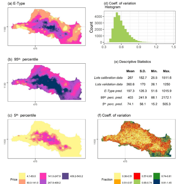
As was described, 100 instances of the logarithm of land values in the GAM were simulated (their back-transformed mean, 95th and 5th percentiles are reported in Fig. 2).
Two important findings can be seen in Fig. 2, perhaps the most important is reported in panels.
(d), (e), and (f): these summarize the uncertainty of the E-Type estimates. The pattern of the coefficient of variation is, approximately, the reverse of the land value predictions (most clearly seen when compared with the E-Type prediction of panel (a)). When contrasted with the density of points (Fig. 1, panel (a)), there is also a clear association. However, the effect of the algorithm can be seen in that the yellow area of low coefficient of variation extends beyond the more urbanized area predicted by large land values (the darker blue and purple intervals of Fig. 2, panel (a), which are also the areas with most sale listings in Fig. 1, panel (a)). The coefficient of variation mostly predicts standard deviations varying between 36 % and 65 % of the mean, suggesting adequately precise measurements (relatively low dispersion in the simulated instances); their distribution tends to be right skewed within this range (shown in the histogram of Fig. 2, panel (d)).

Fig. 2 Fig. 2. Conditional Gaussian Simulation of land value in the GAM (USD per square meter). (a) E-Type prediction (cell-wise mean of simulated instances), (b) 95th percentile of simulated instances, (c) 5th percentile of simulated instances, (d) location-wise coefficient of variation histogram, (e) descriptive statistics of simulated predictions and data, (f) coefficient of variation map.
The second relevant finding of Fig. 2 corresponds to the interpretation of panels (a), (b), and (c): in effect, the E-Type prediction (of panel (a)) is the best estimate of land value; panels (b) and (c) represent higher and lower bound values for this prediction: the land value for 90 % of simulated instances was estimated to lie within the range for each location. An examination of this more detailed set of maps suggests uncertainties may be larger than what the overall measures (of validation, discussed and reported in TABLE I, and of the coefficient of variation) had suggested. By comparing location-wise, for most locations, the upper (95th percentile) or lower bound (5th percentile) shift one category. Given the values involved, this represents around double the back-transformed mean value.
It is also important to understand the quality of the predictions. TABLE I summarizes the validation exercise results. Following the methodological approach, 10 % of the lots data were reserved for validation. For these locations, predictions of land value were generated using (a) the E-Type prediction of the conditional Gaussian simulation (the location-wise mean of all instances) and (b) an ordinary kriging extrapolation, as benchmark. The error was calculated by subtracting the land value per square meter (of the data set) from the back-transformed predicted value. Examining their absolute values, in general, the error terms showed both models underestimated the actual land value.
As can be seen in TABLE I, the E-Type land value prediction is slightly worse than the ordinary kriging: all estimates of error of the E-Type prediction are somewhat larger than the corresponding value for ordinary kriging, as is the range is also smaller. The differences are very small, in general (at least an order of magnitude smaller than the error estimate). It is also worth pointing out that both models have produced very accurate predictions: all mean and median error and RMSE estimates are all less than half of the variable mean (for the land value per square meter of the validation data set, which is reported in Fig. 2).
The predicted pattern of land values per square meter is shown in Fig. 2. The pattern coincides with theoretical expectations and indeed with previous, kriging-based analysis of land values in the GAM from (1): land values are larger (shown in dark blue color) for the centers of San José and Heredia, and the centers of Alajuela and Cartago are also relatively larger than their surroundings. Furthermore, lower values are concentrated on the periphery of the region (rural areas) and the northern zones of Alajuela and Heredia tend to exhibit larger values than those of Cartago and San José.
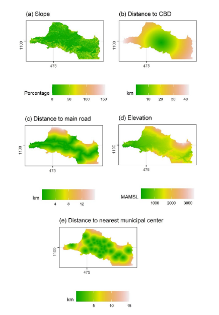
The second objective of this paper, following the estimation of uncertainties, is to explore if these uncertainties respond to regularities in space. To do so, five factors that determine suitability for urban development (and, in consequence, are related to land price formation in urban markets) were considered: slope and elevation, and (Euclidean) distance to the CBD, to the nearest municipal center and to the nearest main road. For each factor, three groups of locations were created (except for elevation, for which only two groups were defined) based on the factor value; group intervals were generally defined based on the variable histograms, although for slope, the group limits are related to statutory building requirements.
TABLE I VALIDATION OF PREDICTION MODELS OF LAND PRICE (USD per square meter)
| Error measure | Prediction model | |
| Conditional Gaussian Simulation (E-Type) | Ordinary Kriging | |
| Root Mean Square Error | 149.4 | 127.7 |
| Mean Absolute Error | 110.7 | 84.3 |
| Median Absolute Error | 82.5 | 56.8 |
| Range of Error | -569.2 – 677.0 | -437.3 – 765.1 |
TABLE II KOLMOGOROV-SMIRNOV STATISTICS FOR DISTRIBUTION OF STANDARD DEVIATION FOR DEVELOPED PREDICTIONS GROUPED BY DETERMINANTS
| Comparison | D Statistic | Prob. |
| Slope | ||
| G1: <30 % vs. G2:>30 % & <50 % | 0.110 | <0.01 |
| G1: <30 % vs. G3:>50 % | 0.137 | <0.01 |
| G2:>30 % & <50 % vs. G3:>50 % | 0.117 | <0.01 |
| Elevation | ||
| G1: <1500 masl G2: >1500 masl | 0.193 | <0.01 |
| Distance to CBD | ||
| G1: <10 km vs. G2: >10 km & < 25 km | 0.412 | <0.01 |
| G1: <10 km vs. G3: > 25 km | 0.583 | <0.01 |
| G2: >10 km & < 25 km vs. G3: > 25 km | 0.178 | <0.01 |
| Distance to nearest municipal center | ||
| G1: <2.5 km vs. G2: >2.5 km & < 7.5 km | 0.364 | <0.01 |
| G1: <2.5 km vs. G3: > 7.5 km | 0.362 | <0.01 |
| G2: >2.5 km & < 7.5 km vs. G3: > 7.5 km | 0.120 | <0.01 |
| Distance to nearest main road | ||
| G1: <1 km vs. G2: >1 km & < 7.5 km | 0.268 | <0.01 |
| G1: <1 km vs. G3: > 7.5 km | 0.409 | <0.01 |
| G2: >1 km & < 7.5 km vs. G3: > 7.5 km | 0.160 | <0.01 |
The Kolmogorov-Smirnov test was used to explore whether the statistical distribution of standard deviation for each group was different from other groups for the same factor. These results are shown in TABLE II and, as should have been expected, all test statistics confirmed the distribution of data of one group is distinct from other groups. On the one hand, there are sufficient simulated locations (over 28000) for even small differences to be significant. On the other, the larger probability of urbanization associated with flatter zones with greater accessibility to urban centralities is also associated with both the point pattern of real estate sales listings (11) –i.e., the sampling density, a key determinant of uncertainty—and the land value itself.

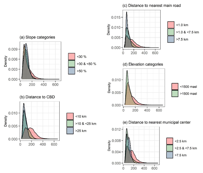
Fig. 3. Fig. 3. Empirical cumulative distribution functions for standard deviation of simulated predictions (square of the log. of USD per square meter). Locations grouped by (a) slope, (b) Euclidean distance to CBD, (c) Euclidean distance to main roads, (d) elevation, and (e) Euclidean distance to nearest municipal center.
How each factor affects uncertainty (measured by the standard deviation of land value of the simulated instances) suggests urban areas have more diverse land values than zones less suitable for urban uses. Fig. 3 shows kernel smoothed empirical distribution densities for the location-wise standard deviation of simulated instances, grouped by the categories that were used in constructing TABLE II. The steeper locations (slopes greater than 50 %) have distinctly larger uncertainty (a sharper peak at higher value of the distribution) than other groups. This same pattern is repeated for all variables: greater accessibilities to urban centralities (the CBD, the nearest municipal center) or the regional transportation network (main roads), represented by the pink density function estimate, have all lower peaks at the lower end of the standard deviation values, suggesting more dispersed values. In general, the intermediate group of factor values (shown in light green, Fig. 3) presents intermediate levels of uncertainty and the group of larger factor values (light blue, Fig. 3), lower levels of uncertainty (the density functions for intermediate groups are less right skewed than those for the larger groups of factor values).
. SYNTHESIS AND DISCUSSION
The analysis of land value patterns extended previous results and it has provided further insights, which have contributed to identify both needs for further study and opportunities for applications to public policy.
The E-Type prediction from the conditional Gaussian simulation was found to marginally improve on ordinary kriging methods. The conditional Gaussian simulation produced, for validation data, slightly better error measures (RMSE, mean, median, and range of error) than ordinary kriging (in the analysis of variations in kriging methods conducted by (1), the different methods tested also resulted in very similar error levels for validation). This result is indeed not surprising, as the simulations are conditional on the variogram, and should more iterations had been simulated, the difference would have likely been smaller. On the other hand, in so far as improvements were generated by the simulations, they were likely related to the improvement of over-smoothing limitations in the kriging predictions (5); but even this feature could have likely been incorporated into the kriging by a careful consideration on the number of neighboring points determining a prediction. Previous exercises of kriging models did find limitations due to this over-smoothing problem that seem to have been improved on by the sequential Gaussian simulation method (in particular, by better modeling the local changes at the peri-urban interface of the region); further work on this issue seems promising.
A distinct advantage of conditional Gaussian simulation is the spatially explicit measures of uncertainty that can be used to explore the limitations of the prediction and to more easily estimate exceedance probabilities (13); this feature is especially useful for land value maps in applied scenarios (for example, when the map predicts land values claimed to be too large by a land owner, this claim can be easily tested). Further work is required on this issue (previous comparisons of models estimated from this data and other data sources suggest systematic underestimation of land values, particularly for taxation purposes (3); while outdated assessments are the simplest explanation, it is also possible that data sources for the models reported in this paper may be also partially skewing the results).
It is further worth noting that the literature has detected over-smoothing problems associated with deterministic methods such as ordinary kriging that can be overcome with simulation. The current focus of this study was not the comparison of conditional Gaussian simulation with other extrapolation predictions; however, this is regarded as a potential area for further investigation.
The estimated uncertainty patterns are inversely related to the predicted land value. A very clear and negative spatial association was identified between the E-Type prediction of land values per square meter and its standard deviation: in the urban central area of the GAM, the highest land values (which coincides both with previous analysis (1) and with theoretical expectations from urban economics) and lowest uncertainties were observed. This finding coincides with previous analysis of the point pattern of real estate listings and its relation to the determinants of suitability for urban land uses (11).
Indeed, the estimated uncertainty was found to decrease with characteristics that identify suitability for urban land use (and thus higher land values). The flatter areas of the GAM, which are also closer to urban centralities (the CBD, main municipal centers), showed much less uncertainty (smaller location-wise standard deviation) than zones further away and at higher elevations and steeper slopes. Therefore, the data set and modeling efforts appear to demonstrate efficiency when predicting urban land values but also present clear limitations if applied to rural land uses of the urban periphery.
Despite its importance, hardly any previous case study reports the use of simulation to understand uncertainty introduced by interpolation into land or property value predictions (unlike physical properties of soils, which are derived from similar point data and for which such analysis seems common). Uncertainty has been reported as variance of kriging estimates (1) or verification through out-of-sample prediction (14), in relation to the mean estimate from this indicator. While theoretical recognition of the possibility to estimate errors and uncertainty in the context of land valuation has been acknowledged (15), actual practice has centered on the accuracy of the mean prediction rather than on explaining its variance. Uncertainty is important for valuation, especially when practical applications are performed (such as tax assessments and potential challenges to these).
In conclusion, the analysis of uncertainties may be critical for improving urban and regional studies (e.g., the impact of new infrastructure or of land use regulations) and land value assessments for tax policy. In this regard, the methods presented have increased robustness (relative to very local estimates) because predictions relatively far away from locations with known values may still benefit from their price information via the spatial dependence encoded in the semivariogram. More importantly, the estimates of uncertainty permit the assessment of the prediction for properties that have not been recently sold in the market (and thus include an inherent check of the prediction which is absent in isolated tax assessment exercises).


