Introduction

Worldwide, air pollution represents one of the greatest concerns because of its proven adverse effects on people’s health (^{WHO, 2016}a). These have been evidenced by a significant number of epidemiological studies developed in recent decades in different parts of the world, which have established a close relationship between the levels of pollutants (gases and particles) concentration in the air and increased mortality as well as hospital admissions for respiratory and cardiovascular conditions, among others (^{Aguiar-Gil et al., 2020}; ^{Cakmak et al., 2018}; ^{Li et al., 2018}; ^{WHO, 2016}b).

One of the mandatory strategies that environmental authorities responsible for ensuring good air quality in their jurisdiction must undertake is the implementation of monitoring networks for atmospheric pollutants (^{Green & Sánchez, 2012}). The data reported by the measurement stations are the input for the formulation of the Integrated Management Plans for Air Quality (planning, implementation, and evaluation (^{AMVA & Clean Air Institute, 2017}). These plans will help achieve acceptable and safe standards for the welfare of inhabitants and ecosystems in general. However, a high percentage of the monitoring networks use expensive technology equipment that require periodic repair, maintenance, services, and specialized calibration procedures. In addition to the high acquisition costs, the operation, transportation, and custody (security) may condition the implementation in areas with difficult access and limited resources, such as energy services and stable communication (^{INE, 2019}).

On the other hand, the complexity in the comprehensive assessment of air quality through the use of these technologies represents a strong limitation, since they are limited to certain chemical compounds and measure pollutants in isolation (^{WHO, 2006}), and they do not allow the establishment of an intrinsic relationship with the biological effect of air pollutants and their long-term consequences on organisms, their communities, and the ecosystem in general (^{Castro et al., 2014}).

Bioindication has been a tool used as a methodological alternative to contribute to the solution of the complex situation that arises in the field of environmental assessment. Moreover, it enables the answering of the questions or uncertainties that stem from the information generated by the conventional monitoring systems on the real physiological and behavioral effects to which organisms are subjected, both in space and time (^{Augusto et al., 2013}; ^{Kienzl et al., 2003}; ^{Van Dijk et al., 2015}). Therefore, the use of different groups of organisms as indicators has been consolidated as an adequate alternative to evaluate the effect that may be derived from the deterioration of air quality in a territory under study. Due to their anatomical, morphological, and physiological characteristics, the lichen has been used as a bioindicator with successful results. Moreover, as they are widespread worldwide, lichens allow the determination of the involvement degree when they are exposed to dangerous substances, as in the case air pollutants, allowing the classification of some species as sensitive and others as tolerant (^{Anze et al., 2007}; ^{Cleavitt et al., 2015}; ^{Käffer et al., 2011}; ^{Jovan, 2008}).

Lichens are intimate and long-lasting symbioses of photosynthetic algae or cyanobacteria and heterotrophic fungi (^{Piercey-Normore & DePriest, 2001}). This symbiotic relationship is related to their tolerance and / or sensitivity, so they can be used as bioindicators (^{Llop et al., 2012}). Since the techniques for the implementation of their use as bioindicators can be considered simple and low-cost maintenance, lichens have great strengths as an instrument for the diagnosis of air quality (^{Correa-Ochoa et al., 2020}; ^{Hawksworth et al., 2005}; ^{Salcedo et al., 2014}). Furthermore, they define air quality levels with greater precision, establishing limits that are difficult to be detected by conventional systems and allowing the determination of the degree of impact on humans, given that they are exposed to the same complex mixture of air pollutants (^{Castro et al., 2014}).

The excellent results that the different biomonitoring programs with lichens have produced have served as an argument to integrate them into environmental assessment strategies of national protocols in countries such as England, Germany, the United States and the Netherlands (^{Anze et al., 2007}; ^{Käffer et al., 2011}; ^{Monge-Nájera et al., 2002}). In this regard, the evaluation of the spatial behavior patterns of these air quality bioindicators has allowed the establishment of associations between their diversity, such as their bioaccumulation capacity, their relationship with the state of contamination in some areas, as well as their relationship with some diseases (^{Cislaghi & Nimis, 1997}; ^{Pollard et al., 2015}; ^{Ribeiro et al., 2016}; ^{Yatawara & Dayananda, 2019}).

The articulation of current systems for measuring air quality and the use of bioindicators, represents an alternative that allows a better knowledge of pollution, especially in cities like Medellín that register areas with significant air quality alterations and that have a robust monitoring network for the diagnosis of air quality but do not have qualitative tools to assess its impact on living beings. In this sense, this study aims to evaluate the changes in the composition of corticulous lichen communities as a response to various stress factors in areas with different levels of air quality. This was achieved through the quantification of lichen richness and coverage, mapmaking, and the determination of relationships among these parameters, land uses, and distance to roads in the different biomonitoring areas, located in Medellín city.

Materials and methods

Study site: Medellín city is located in the central mountain range of the Colombian Andes (Fig. 1A and Fig. 1B) at an average height of 1 450 m above sea level; it is centered in a deep (1 km) and narrow (10 km on average) valley called Valle de Aburrá. The city has a temperate-dry climate, with average annual temperature values of 22.5 °C, precipitation of 1 685 mm, relative humidity of 67 % (^{IDEAM, 2018}a), and a predominant direction of the winds from North to South in the axis of the valley ^{(IDEAM, 2018}b). During recent years, the levels of air pollution in the valley have generated great concern; especially the PM_2.5 particulate material (^{Gaviria et al., 2011}; ^{MADS, 2012}). This, in addition to the valley´s topography and the local and regional meteorological conditions that vary throughout the year, favors episodes of atmospheric stability (mainly in March-April and October-November) that influence the pollutants dynamic dispersion (^{Correa et al., 2009}). Considering the risk that air pollution has on people’s health, Valle de Aburrá has one of the most robust and advanced air quality networks in the region (BID, 2016) that is integrated into the Sistema de Alerta Temprana del Valle de Aburrá (SIATA).

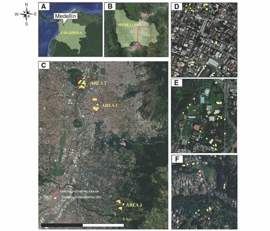
Fig. 1 Biomonitoring area. A. Study area location in Colombia, B. Study area location in the City of Medellín, C. Biomonitoring areas, D. Area 1, E. Area 2, F. Area 3. (Coordinate system - WGS_1984). 

Biomonitoring areas: This study was conducted in three biomonitoring areas (Fig. 1C) that present differences in their sources of air pollutant emission as well as physical and environmental conditions. Area 1 is located in the center of the city in a commercial and institutional sector, comprises emissions mainly due to vehicular traffic with roads where urban, inter-municipal, and private and public transport converge in the city. It has little vegetation with isolated trees, located mainly on platforms that are part of the urban planning of the area (Fig. 1D). On the other hand, Area 2 is characterized by heterogeneous conditions, combining exposure to high vehicular traffic and large vegetation areas (Fig. 1E). This area is located inside the Universidad Nacional de Colombia, which has a great number and diversity of tree species. Finally, Area 3 is located in an area with different characteristics from the previous ones (Fig. 1F). It is defined by predominant vegetation and scarce emissions of pollutants of industrial origin. This is an area of important contrast with land uses mainly forestry.

General air quality of the biomonitoring areas: The annual average concentrations of PM_2.5 reported by SIATA for the year 2018 were inserted using Spline, a tool of ESRI’s ArcGis® software to assign the air quality associated with the biomonitoring areas to generate isoconcentration maps of this pollutant. Subsequently, an estimated average value was obtained for this pollutant in each of the areas from the maps obtained and using the spatial analyst tools (Extract values to points) of ESRI’s ArcGis® software.

Lichen species mapping, collection, identification and area determination: In each of the three biomonitoring areas, 28 to 30 phorophytes were sampled (without species differentiation). The field work focused on the identification of the number of lichen species and on the mapping of the specific coverage of lichens. Moreover, it followed the methodology proposed by ^{Monge-Nájera et al. (2002}), in which a transparent film of polyethylene terephthalate (acetate) of 50 cm × 100 cm and 0.4 mm thickness was fixed on the bark of the tree at a height of 50 cm, measured from the ground level up to the lower edge of the acetate on the side where the greatest presence of lichens was evident (Fig. 2A).

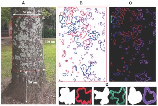
Fig. 2 Lichen mapping in phorophytes, and counting and inventory of lichen areas A. Acetate location in each phorophyte B. Acetate digitized with a metric scale C. Color identification. D. Quantification of the area. 

Subsequently, the outer contour of the lichen spot (no matter how type of thallus they have) was outlined with a fine-tipped marker using a different color for each lichen species (Fig. 2B). Each acetate was digitized at a 1:1 scale in the presence of a metric pattern and was stored in digital “.tiff” format. Then, each digitized image was processed using ARLIQ® software that determines the inventory of lichen cover (Fig. 2C and Fig. 2D) and the number of lichen species (lichen richness per phorophyte). The design of this software emerged as a tool to conduct a research project by GIGA and GEPAR groups of the Facultad de Ingeniería de la Universidad de Antioquia (UdeA).

Representative specimens were collected according to the methodology proposed by ^{Chaparro & Aguirre (2002}) and then the characterization of the lichen species was performed using the methodology of ^{Orange et al. (2001}).

^{Simpson Index and resistance factor: The Simpson Index (Simpson, 1949}) was calculated for different intervals of distances (0-50 m, 50-100 m, 100-150 m, >150 m) in each area, with respect to the roads (Area 1 and 2) or respect to the forest area (Area 3). Likewise, the resistance factor, were calculated for the same distance intervals. This factor establishes the degree of sensitivity of the species, assuming that contamination reduces its diversity and the sensitivity of a specie depends on its representativeness in the environment in which it is found (^{Jaramillo & Botero, 2010}).

Data analysis: Kruskal-Wallis test were used to evaluate whether statistically significant differences were present between the richness and coverage medians of the mapped phorophytes in the biomonitoring areas and Mann-Whitney U were used to do paired comparisons between richness and coverage medias for different levels of these factors. Furthermore, the Moran index was also used to determine the possible existence of spatial clustering patterns of richness and coverage values.

The richness and lichen coverage values obtained for each sampling unit were interpolated using two mathematical algorithms: Inverse Distance Weight (IDW) and Radial Basis Function (Spline). Geostatistical Analyst® tool of ESRI’s ArcGis® software was used to perform all the analyses. The algorithm with the best performance was chosen to represent the distribution of lichens.

The performance of each interpolation algorithms was performed using the leave one out cross validation method (^{James et al., 2013}), and then calculating the index of agreement (IOA), root mean square error (RMSE), and the RMSE standardized (RMSS). The best mathematical performance algorithm comprised the lowest RMSE and an RMSS and IOA closer to 1 (^{Chai & Oceanic, 2015}; ^{Szpiro et al., 2007}; ^{Willmott et al., 2012}).

The relationships between intra-area lichen richness and cover, land use, and roads distances were evaluated using the Spearman correlation coefficient. The information regarding the road network and land use was downloaded from the official public website GeoMedellín (^{Alcaldía de Medellín, 2021}). The phorophytes distances to the roads and soil types were calculated using the Euclidean Distance tool of ArcGis® Software; the number of lichen species was calculated for different intervals of distances (0-50 m, 50-100 m, 100-150 m, >150 m) in each area, with respect to the roads (Area 1 and 2) or respect to the forest area (Area 3). Likewise, the ^{Simpson index (Simpson, 1949}) were calculated for the same interval distances and the resistance factor of each lichen specie (^{Correa-ochoa et al., 2020}) were calculated for the same distance intervals. Finally, a Kruskal-Wallis test was used to determine the existence of statistically significant differences in the resistance factor between distance intervals, and the Mann-Whitney U were used to do paired comparisons between the resistance factor medias in the different distance intervals. All analyses were carried out using software RStudio version 3.6.3 (^{RStudio Team, 2020}).

Results

Air quality in biomonitoring areas: Fig. 3A shows the air pollution patterns associated with the annual average of PM_2.5 for the study area in 2018. The highest estimated concentration is in Area 1 with 26.93 µg/m³, followed by Area 2 with 21.29 µg/m³, and finally, Area 3 with 18.84 µg/m³ (Fig. 3B).

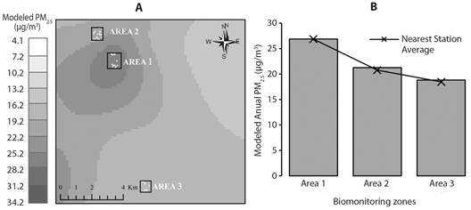
Fig. 3 A. Modeled Annual Concentration of PM_2.5 (general error of Spline interpolator with an error of ± 4.97 µg/m³) B. Modeled Annual Concentration in the biomonitoring areas. 

Lichen diversity, coverage, and richness in the biomonitoring areas: 110 species of lichens were identified. The most frequent was Phaeophyscia chloantha (Ach.) Moberg, that was present in 33 of the 86 phorophytes evaluated in all areas, followed by the Physcia poncinsii Hue that was in 28 phorophytes. The highest number of species was in Area 1 with 84, followed by Area 2 with 44, and finally, Area 3 with 23. In Area 1, Phaeophyscia chloantha (Ach.) Moberg (21 of the 30 phorophytes) and Candelaria concolor (Dicks.) Arnold (20 of the 30 phorophytes) were dominant and for Area 3, Candelaria fibrosa (Fr.) Müll. Arg (12 of the 26 phorophytes) was dominant.

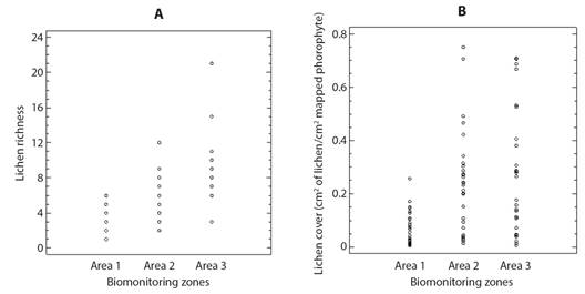
According to the Kruskall-Wallis test, statistically significant differences were present in at least one of the richness (P < 0.05) and coverage (P= 0.00) medians in the biomonitoring areas, and the paired comparisons (Mann-Whitney U test) for richness values in the biomonitoring areas, the test indicates statistically significant differences in the medians for all the pair comparisons evaluated. Also, PM_2.5 values are negatively correlated with richness (R= -0.7) and coverage (R= -0.4) in the biomonitoring zones (Fig. 4A). Similarly, for coverage values in the biomonitoring areas indicated significant differences between areas 1-2 and 1-3 (P < 0.05 in both cases); while no statistically significant differences were found for this variable in areas 2-3 (P= 0.88) (Fig. 4B).

Fig. 4 A. Lichen richness B. Lichen cover. 

Performance of spatial interpolation algorithms and spatial patterns of lichen richness and lichen coverage: The results of the Moran Index indicate that clustering patterns (With z values > 0) are presented in the observations of richness (z= 6.7, P= 0.00) and coverage (z= 3.65, P= 0.00) and there is spatial autocorrelation of the observations with P-values < 0.05, indicating that there is a probability of less than 1 % that these clusters are the result of chance.

The Spline model was the chosen model, since, in the case of richness, it presented a lower RMSE and an RMSS and IOA closer to one in relation to the IDW model. In the case of coverage, it presented an RMSS closer to one and a lower RMSE (Fig. 5A). The errors associated with the interpolation model of the richness and coverage values can be observed in Fig. 5B and Fig. 5C, where the error associated with the interpolation model is 2.3 for richness and 0.18 cm² of lichen/cm² of mapped phorophyte for coverage.

Fig. 5 A. Spatial interpolators comparison Spline and IDW B. Predicted values adjustment vs. richness observed values C. Predicted values adjustment vs. observed values for coverage (cm² of lichen/cm² mapped phorophyte).  

Fig. 6 shows the land uses and pathways in each biomonitoring area (Fig. 6A, Fig. 6B and Fig. 6C). Spatial distribution patterns of the lichen richness (Fig. 6D, Fig. 6E and Fig. 6F) and coverage values (Fig. 6G, Fig. 6H and Fig. 6I) using the Spline spatial interpolation algorithm. According to the scales of the color patterns in the figure, it can be observed that the richness and coverage of lichens was lower in zone 1 compared to zones 2 and 3. Likewise, the zone that presented a higher value of richness and coverage was zone 3.

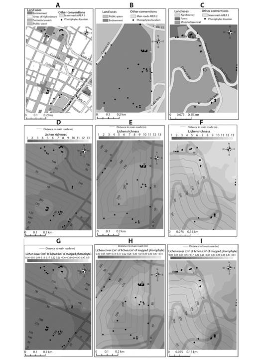
Fig. 6 Spatial distribution patterns of lichen cover and richness values using the Spline interpolation, and land uses and roads in each biomonitoring area. A. Area 1 land use and roads B. Area 2 land use and roads C. Area 3 land use and roads D. Area 1 richness and main roads distances E. Area 2 richness and main roads distances F. Area 3 richness and main roads distances G. Area 1 coverage and main roads distances H. Area 2 coverage and main roads distances I. Area 3 coverage and main roads distances. 

Lichen coverage and richness intra areas: A positive correlation was found between richness and distance to main roads (Fig. 7A) in Area 1 (R= 0.58). In the case of coverage, no significant relationship was found with respect to the distance to main roads (R= 0.1338, P= 0.47) in this area (Fig. 7B). In Area 2 we found a positively correlation (R= 0.5) between lichen richness and distance to roads (Fig. 7C). In the case of coverage (Fig. 7D), no significant relationship was found with respect to the distance to roads at this site (R= 0.04). Finally, in Area 3 richness values were negatively correlated (R= -0.5) with the distance to the forest (Fig. 7E). For the case of the coverage (Fig. 7F), a moderate-low relationship was found (R= -0.39). Note: For Area 3 richness and cover values were correlated with distance to forest zona, given that the phorophytes sampled in this area were located on the sides of the roads (distance to roads = 0 m) and not inside the forest area to avoid edge effects that could generate erroneous interpretations in the data analysis.

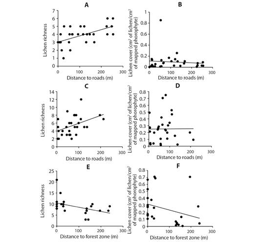
Fig. 7 Lichen richness and coverage in relation to the distance to roads or in relation to distance to forest region. A. Area 1 richness and main roads distances B. Area 1 cover and main roads distances C. Area 2 richness and main roads distances D. Area 2 cover and main roads distances E. Area 3 richness and forest zone distances F. Area 3 cover and forest zone distances. 

Species diversity estimators and resistance factor by distance intervals: Fig. 8 shows de number of species and the Simpson index for the areas in the different distance intervals to roads (Area 1 and 2) or to the forestry area (Area 3). The obtained results for area 1 (Fig. 8A) showed an increase in the number of lichen species as the distance intervals are further from the roads, presenting the highest number at distances > 150 m with a total of 18 lichen species. Likewise, the Simpson index was higher as the distance to the road increases. On the other hand, area 2 (Fig. 8B) presented the highest number of species in the distance to roads between 50 and 100 m with a total of 31 species; thereafter, the richness decreases when the distance to the roads increases, going from having 23 species between 100 and 150 m to 11 at distances > 150 m. Regarding the Simpson index, its highest values were presented in the distance intervals between 50-100 m and between 100-150 m. Finally, in area 3 (Fig. 8C), the highest number of species occurred in the distance interval between 0 m and 50 m from the forest zone with a total of 90 species and in that same distance interval the highest value of the Simpson index was presented.

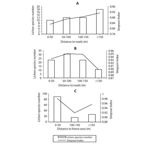
Fig. 8 Lichen species richness and Simpson Index in relation to distance to roads for A. Area 1 and B. Area 2 or C. In relation to distance at forest region for Area 3. 

According to the results of the Kruskal-Wallis test there were statistically differences in the resistance factor for the different distance groups. For area 1 the resistance factors of the species located at distances > 150 m were higher (Fig. 9A) and the Mann-Whitney U test established that they were different from those reported for the other distance intervals. Likewise, this test established that there are no differences in the resistance factors of the species located in the distances between 0-50 m, 50-100 m and 100-150 m.

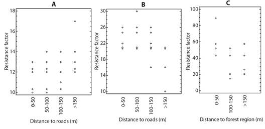
Fig. 9 Q Factor in relation to the distance to roads A. Area 1 and B. Area 2 or in relation to distance to forest region C. Area 3. 

On the other hand, for area 2, there were statistically significant differences in the resistance factor for the different distance groups (P= 0.000) and the Mann-Whitney U test identified two different homogeneous groups that establish that the resistance factor registered for the distance groups of 0-50 m, 50-100 m and 100-150 m does not present differences and that the resistance factor of the lichen species at distances > 150 m was different from that of the other distance groups. In this sense, for this distance interval it was found that the resistance factors were lower (Fig. 9B). Finally, the resistance factor calculated for the lichen species in the different distance intervals for area 1, present statistically significant differences (P= 0.000), and three different homogeneous groups were identified according to the Mann-Whitney U test. Therefore, the resistance factor is statistically different in the three distance ranges. In this sense, the resistance factor was higher for the species found closer to the forest zone (0-50 m) (Fig. 9C).

Discussion

The results showed the presence of lichen species that indicate the state of intervention of the ecosystems. Species like P. chloantha has been documented in previous studies as a resistant specie, commonly found in strongly anthropogenically altered environments (^{Skirina & Kozhenkova, 2018}). On the other hand, ^{Gupta et al. (2017}) found that some species belonging to the genus Phaeophyscia are considered as indicator species in urban areas due to their ability to bioaccumulate heavy metals. Still, the C. concolor species has been informed as a tolerant species to contamination, as reported in studies such as ^{Ochoa-Jiménez et al. (2015}) and ^{Saenz et al. (2007}). Likewise, the species C. fibrosa was dominant in Area 3; this species was classified by ^{Gonzales Vargas et al. (2016}) as a species sensitive to contamination.

Areas with better air quality had more lichen richness and coverage, these findings coincide with previous studies that found relationships between lichen diversity and air quality in different areas (^{Gombert et al., 2004}; ^{Käffer et al., 2011}). Furthermore, the richness and abundance of lichens significantly respond to the concentrations of PM_2.5 in a linear and negative way, so that the lichens in the study areas are clear indicators of the concentration of particles, and according to ^{Varela et al. (2018}), they can be used to estimate PM_2.5 concentrations in areas that do not have monitoring stations.

At the zonal level, patterns of relationships were identified between observations of coverage and richness as well as the environmental and pollution characteristics of the zones. In Area 1, the contamination characteristics result in low richness and coverage values, and therefore, the establishment of lichens in the area depends on the tolerance of the species, their anatomy, their water retention capacity, and their mechanisms for detoxification of adverse effects, and according to experts, it may be modified by different environmental conditions and by the distribution area (^{Nimis et al., 1990}).

Area 2 presents a homogeneous environment in terms of land use. Hence, variations and groups of coverage and richness could be associated with roads as their main source of pollution. For this zone, the richness increases as the sampled phorophytes are further from the surrounding pathways. This result is consistent with reports such as those presented by ^{Perlmutter et al. (2017}) and ^{Will-Wolf et al. (2015}). Note that there are responses related to changes in the composition of lichen communities. Moreover, the spatial heterogeneity of lichens in an area is greatly related to its land uses; thus, the air quality indexes established using lichens present higher values in garden areas and lower values in the vicinity of vehicular traffic. This coincides with the findings found by ^{Ribeiro et al. (2016}). Likewise, the Universidad Nacional de Medellín (located in Area 2) is characterized by having green corridors in its periphery, which makes the environment conducive to generating edge effects in microclimate conditions for the establishment of lichen communities (^{Aragón et al., 2015}). Furthermore, these green corridors help reduce pollution levels (^{Hagler et al., 2011}).

In area 3, richness values presented greater responses for phorophytes that were within and near the forest zone. These relationships can be explained as the result of the adaptation of lichens to the pollution gradients that occur as the phorophytes sampled are located further away from the urban-rural zone and approach or locate in the forest zone. With respect to the latter, ^{Barreno and Pérez-Ortega (2003}) state that the proximity to forest mass structures is a key factor that should be considered, given that in or near forest areas, different types of microenvironments can be created that are immediately detected by the lichens and that can contribute to the creation of adequate conditions for the establishment of such communities. In addition, the presence of green areas increases humidity and is considered a barrier to air pollutants (^{Barreno & Pérez-Ortega, 2003}).

In general, lichen richness presented better relationships with respect to the environmental and pollution conditions of the different areas. This may be attributed to the fact that this indicator may present a greater sensitivity to the disturbances detected by lichens. In addition, the richness of lichens is considered a good element to determine for describing general environmental state characteristics of an area (^{Varela et al., 2018}).

The obtained results indicate that the corticulous lichen communities present a response to environmental factors and pollution in biomonitoring areas. Moreover, it yields the knowledge of the quality of the environment with a high spatial resolution. This knowledge can be used as a warning to detect ecosystem damage and can provide crucial information regarding the generation of policies for land planning and ecosystem conservation. Therefore, these bioindicators can represent an environmental pillar toward sustainable development. Bioindication can answer crucial questions about risk without the need for an elaborate chemical analysis. Lichens can be used as warning systems for environmental problems, evaluation of the environmental health of an ecosystem, among others, since the lichen species disappearance may be more tangible than the “parts per trillion” of a chemical (^{Kienzl et al., 2003}). Thus, establishing variations in the lichen communities between and within areas that allowed classifications and determining effects according to their exposure to contamination sources (routes) and land uses are possible; both are important responses for the study of air quality (^{Ulshöfer & Rosner, 2001}).

Relationships in composition of lichen communities associated to local pollution sources exposure and its extent limits were determined. This information may have great relevance in public health studies, since human beings located in these areas are exposed to the same complex mixture of pollutants to which lichens have been exposed to in this study. Based on the above, studies such as that of ^{Cislaghi and Nimis (1997}) highlight the importance of associating the monitoring of the diversity of lichens with the mortality rates. This finding represents a valuable tool for the knowledge of the environmental health in cities like Medellín that register areas with significant air quality alterations and that have a robust monitoring network for the diagnosis of air quality but do not have qualitative tools to assess its impact on living beings.

Ethical statement: authors declare that they all agree with this publication and made significant contributions; that there is no conflict of interest of any kind; and that we followed all pertinent ethical and legal procedures and requirements. All financial sources are fully and clearly stated in the acknowledgements section. A signed document has been filed in the journal archives.