


 English (pdf)
 Article in xml format
 Article references
 Send this article by e-mail
 Cited by SciELO
  Similars in
SciELO
Similars in
SciELO  uBio
uBio 
 Permalink
Copepods are an important planktonic group, and account for most of the total biomass and species diversity in pelagic marine ecosystems. In coastal and oceanic regions of the Eastern Tropical Pacific off Mexico (ETPM), they have been reported to comprise around 66-76 % of total zooplankton abundance (Franco-Gordo et al., 2015; PelayoMartínez et al., 2017). Subsequently, they greatly contribute to zooplankton production and energy transfer to higher trophic levels. In the ETPM, copepods are exposed to a complex mix of environmental conditions, such as seasonal changes in the water column, principally regulated by the summer/fall poleward Mexican Coastal Current (MCC) (Lavín, Beier, Gómez-Valdés, Godínez, & García, 2006; Salas, Gomis, Olivos-Ortiz, & García-Uribe,
2006; Gómez-Valdivia, Parés-Sierra, & FloresMorales, 2015), and a winter/spring tropical extension of the California Current (Salas et al., 2006; Godínez, Beier, Lavín, & Kurczyn, 2010). Other important hydrological characteristics include mesoscale eddies, which are usually present year-round with seasonal variations (Kurczyn, Beier, Lavín, & Chaigneau, 2012), winter/spring coastal upwelling (TorresOrozco, Trasviña, Muhlia-Melo, & OrtegaGarcía, 2005; López-Sandoval, Lara-Lara, Lavín, Álvarez-Borrego, & Gaxiola-Castro, 2009) and an extremely shallow upper layer of the oxygen minimum zone (OMZ, 9.0 µmol L-1) which reaches depths of ~50 m along the coast (Zamudio, Hurlburt, Metzger, & Tilburg, 2007; Cepeda-Morales, Beier, Gaxiola-Castro, Lavín, & Godínez, 2009). These environmental conditions make this area a dynamic transitional environment that influences patterns of temperature, dissolved oxygen, and primary and secondary productivity (Ambriz-Arreola, Gómez-Gutiérrez, Franco-Gordo, & Kozak, 2015; Kozak, Franco-Gordo, Palomares-García, Gómez-Gutiérrez, & Suárez-Morales, 2017; Pelayo-Martínez et al., 2017).
Distribution, feeding and reproduction of zooplankton are influenced by abiotic factors like bathymetry, thermocline depth, temperature, primary productivity and food availability. These factors are in turn modulated by dynamic structures such as eddies (cyclonic and anticyclonic), upwelling events and filaments, which due to their 1-100 km size are referred to as dynamic mesoscale structures (DMS). These DMS are usually caused by gravity, density gradients and wind forcing, and provoke a resuspension or sinking of particles and organisms, which generates patches of organisms according to hydrological conditions, reflected in the abundance of distinct zooplankton groups (Pelayo-Martínez et al., 2017). Within the zooplankton, copepods form important prey for the most common fish larvae found in the ETP off Mexico (ETPM), Bregmaceros bathymaster (Siordia-Cermeño, Sánchez-Velasco, Sánchez-Ramirez, & FrancoGordo, 2006; Davies et al., 2015). This permits the establishment of complex food webs with a seasonal component and ecological importance for a region considered to be oligotrophic, but which supports a variety of artisanal fisheries (Rojo-Vázquez et al., 2008).
Previous studies about the variability of copepod communities in the ETPM were either carried out exclusively in coastal sites (Kozak, Franco-Gordo, Suárez-Morales, & PalomaresGarcía, 2014; Jiménez-Perez, 2016) or over a greater spatial range but restricted to a single period without seasonal replicates (Chen, 1986; López-Ibarra, Hernandez-Trujillo, Bode, & Zetina-Rejon, 2014). We hypothesize that variability in the abundance and diversity of the copepod community was principally driven by seasonal mesoscale activity (upwelling and eddies) and the moderate El Niño-La Niña event, which impacted the tropical Pacific during this period. The goal of this study was to provide the first analysis of seasonal changes in the copepod community structure of the ETPM through the El Niño-La Niña transition of 2010, and to examine the relationship between the distribution of copepods in the ETPM and environmental variables.
Materials and methods
Sampling: Three oceanographic cruises were carried out from 15-27 January (Jan), 25 May- 4 June (May), and 18-29 October (Oct) 2010. Twenty-one stations were sampled in each cruise distributed along three transects parallel to the coast at a distance of 10 nm, 50 nm and 100 nm from Cabo Corrientes, Jalisco to Maruata, Michoacán, Mexico (Fig. 1). Six samples were unavailable for analysis (Jan 3, 4, EX2; Mar 9, 13, 14; Oct 11, 15, EX1), leaving 18 stations for each of the three sampled months. Sampling methods are as in PelayoMartínez et al. (2017). Briefly, oblique zooplankton tows were performed during daytime and nighttime at each station, from 200 m depth or as deep as possible, using a bongo net with a mesh size of 505 µm, and with a mouth opening of 0.6 m in diameter (Smith & Richardson, 1977). A calibrated flowmeter was attached to the mouth of the net to estimate the amount of water filtered. Samples were fixed in a 4 % formalin solution buffered with sodium borate (Griffiths, Fleminger, Kimor, & Vannucci, 1976). Before zooplankton sampling, temperature and salinity profiles were recorded at each station using a CTD (SBE-19 plus), with the depth of each cast ranging from 75 to 500 m depending on the bathymetry of each station. Water samples were collected using Niskin bottles at depths of 200, 150, 100, 75, 50, 25, 10 and 0 m and analyzed for inorganic nutrients (NO3 -+NO2 -, NH4 +, PO4 -3, Si(OH)4) using an auto-analyzer Skalar San Plus II and chlorophyll a (Chl a) with a Perking Elmer’s UV/Vis spectrophotometer following the techniques proposed by Grasshoff, Kremling, and Ehrhardt (1983) and Strickland and Parsons (1972). In accordance with Talley, Pickard, Emery, and Swift (2011), altimetry data from the AVISO program (http://www.aviso.altimetry.fr/en/data.html) were processed to identify sea level anomalies and geostrophic currents (with 1/3° resolution); both parameters were plotted using ®MATLAB 8.1.0.604 software.

Fig. 1 Study area in the central Mexican Pacific during January (Jan), May-June (May), and October (Oct) 2010.
Species identification: In the laboratory, samples were fractioned using a Folsom plankton splitter to obtain final sub-samples of 300500 specimens (Harris, Wiebe, Lenz, Skjoldal, & Huntley, 2000). Adult copepods were identified to species level and copepodites were identified to family level. Although probably under-sampled as a group, cyclopoid copepods were still identified to species level (except in the case of Oncaea spp., which due to uncertainty were identified at the genus level only). We included these organisms as they are part of the total biomass of the larger size fraction of copepods. Identifications followed the keys of Palomares, Suárez, and Hernández-Trujillo (1998) and Razouls, de Bovée, Kouwenberg, and Desreumaux (2005-2017); when necessary other specialized keys were used.
Data analysis: Standardized copepod abundance data were explored to detect outliers, then Log10 [x+1] transformed before performing statistical or multivariate analyses to decrease the variance of the data set and to avoid violating assumptions of normality, except for non-parametric analyses which do not require such transformations. Because zooplankton samples were taken during both night and day, an analysis of variance (ANOVA) was first used to check for significant differences between total copepod abundance and time of sampling. Daytime and nighttime classifications were based on the time of sunrise and sunset during each sampling period. Daytime = 1 hr before sunrise to 1 hr after sunset. Nighttime = 1 hr after sunset to 1 hr before sunrise. No significant differences were found, so samples were defined a priori to statistical analysis by month and inshore (0, 4, 8, 12, 17, 19, EX1) or offshore (remaining stations). Mean abundance and abiotic data of the different sampling periods Jan, May and Oct) were compared using an ANOVA to determine overall changes in the region. If significant results were detected, a Tukey’s test was used post hoc to define the differences. The ANOVA and post hoc analyses were calculated using Statistica 10.0 software (Stat Soft).
A cluster analysis (CA) was performed to define copepod assemblages using the Sorensen distance measure and β-flexible linkage method (β = 0.25), followed by a multi-response permutation procedure (MRPP) to test the significance of the resulting groups. The similarity percentage (SIMPER) was used to identify the species that account for 90 % of abundance of the species/families that made up the groups defined by the CA. An indicator value analysis (IVA) was also applied to determine which species could serve as indicators of certain hydrological conditions based on the CA groups (Dufrêne & Legendre, 1997). The IVA provides the percentage of indication by combining values for relative abundance and relative frequency, with results ranging from zero (no indication) to 100 (perfect indication). Canonical correspondence analysis (CCA) defined the relationships between species assemblages and environmental characteristics in multivariate space. The environmental (explanatory) matrix in the CCA consisted of surface (0-50 m) and subsurface (75-200 m) means of temperature, salinity, Chl a (mg m-3), dissolved oxygen (DO; µmol kg−1), nitrate+nitrite (µM), ammonium (µM); phosphate (PO3- 4¸ µM), and silica (µM). The biological (response) matrix consisted of 76 species and copepodite taxa. To test for the significance of the first ordination axis and all canonical axes together, a Monte Carlo permutation test (499 permutations) was applied. Rare species, defined as those appearing in < 5 % of samples, were not included in either CA or CCA analyses. Multivariate analyses were carried out using PC-ORD v.4 software (McCune & Mefford, 1999).
Temperature/Salinity profiles of the water masses found in the study area during the three oceanographic cruises were created by integrated plots using ®MATLAB 7.11 software according to the limits proposed by Portela et al. (2016). Based on the environmental variables that explained most of the variability seen in the sample distribution, contour maps representing the horizontal distribution of Chl a (0-50 m), salinity (0-50 m), NO3 -+NO2 - (0-50 m), and NH4 + (75-200 m) were created using Surfer 11 software.
Results
Environmental conditions: The survey period of the present study included the second half of the 2009-2010 El Niño (EN, Jan 2010), the neutral transition period (May 2010), and the first half of the 2010-2011 La Niña (LN, Oct 2010). [The entire ETP experienced an ENSO cycle from 2009-2011 (http://www.cpc. ncep.noaa.gov/products/analysis_monitoring/ensostuff/ensoyears.shtml)]. The water masses in the upper water column during the three periods were primarily characterized by Tropical Surface Water (TSW), Gulf of California Water (GCW) and a high proportion of transitional water as a result of the confluence of those water masses in the region. In the intermediate layer, the water column was dominated by Subtropical Subsurface Water (StSsW). Jan samples were mostly TSW, probably due to the effect of EN. May samples were dominated by transitional waters and a slight influence of GCW. Oct samples were more varied, with a stronger influence of GCW and a slight influx of California Current Water (CCW) (Fig. 2). The mean temperature of the surface layer (0-50 m) was warmest during Jan (26.8 °C), which coincided with the expanded mixed layer depth (MLD 45.8 m), the highest value of the Multivariate Enso Index (MEI 1.52) and the lowest value of the Coastal Upwelling Index (CUI; https://www.pfeg.noaa.gov/products/PFEL/modeled/indices/upwelling/NA/data_download.html).
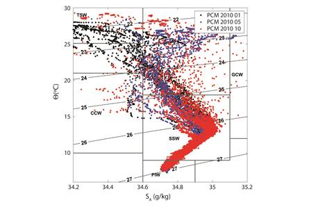
Fig. 2 Temperature/Salinity profiles of the water masses found in the study area during the three oceanographic cruises of 2010. TSW = Tropical Surface Water; CCW = California Current Water; StSsW = Subtropical Subsurface Water; GCW = Gulf of California Water; PIW = Pacific Intermediate Water.
Eddy processes: Geostrophic currents showed seasonal variations in direction and intensity, along with a subsequent increasedecrease of temperatures (Fig. 3A, Fig. 3B and Fig. 3C). Jan was dominated by a geostrophic flow from the south. A very weak cyclonic eddy was apparent near the center of the surveyed area (Fig. 3A), but it had little effect on surface temperatures, which were relatively high and uniform across the region in the upper water column (0-50 m). A cyclonic eddy in May showed a much stronger flow (Fig. 3B) and resulted in cooler temperatures at the core. During this period a geostrophic current parallel to the continent was apparent; it is probable that the effect of movement near the coast along with the topography of the platform generated internal waves. This could have generated a point of lifting of the water column, resulting in lower temperatures and brief episodes of primary productivity in the surface waters near the coast. In Oct a large anticyclonic (warm core) eddy was apparent in the central study area, with a much smaller cold core eddy directly below it (Fig. 3C).
Fig. 3 Contour maps of important environmental variables in the region during the three study periods. Months are January (Jan) (A, D, G, J, M); May-June (May) (B, E, H, K, N) and October (Oct) (C, F, I, L, O). Note the different color scales for each variable.
Upwelling and Chl a: Over the entire study area, nutrient concentrations at surface (0-50 m) and sub-surface (75-200 m) depths were averaged and analyzed for differences between surveyed periods (Table 1), and several of the most relevant variables were expressed as contour maps (Fig. 3). Both 0-50 m and 75-200 m ammonium values were highest in Jan. Values of 0-50 m nitrates+nitrites (mineralized nitrogen found in deeper waters), silicates and phosphates were significantly higher in May, representative of upwelling processes along the coast as well as in the large cyclonic eddy (Fig. 3B and Fig. 3K). Jan showed very low nitrate+nitrite values over the entire region, except for a slight increase near the weak cyclonic eddy (Fig. 3A and Fig. 3J). Downwelling conditions dominated during Jan, as shown by significantly higher temperatures, ammonium and DO concentrations, and a deeper MLD than the other two periods (Table 1). The monthly mean of daily CUI values corroborated that coastal upwelling processes were highest in May, were present during Oct, and absent during Jan (Table 1). Despite the lack of active upwelling conditions, very high 0-50 m Chl a concentrations were observed at an inshore station during Jan (Fig. 3D), resulting in significantly higher concentrations than in May and Oct (Table 1).
Table 1 Environmental variable mean for three periods in 2010
| Variable 1 | Jan (SE 2 ) | May (SE 2 ) | Oct (SE 2 ) | p | F | post hoc | ||||||
|---|---|---|---|---|---|---|---|---|---|---|---|---|
| T 0-50 | 26.8 | (0.21) | 23.9 | (0.34) | 23.5 | (0.54) | < 0.001 | 21.36 | J > All | |||
| T 75-200 | 15.24 | (0.48) | 13.83 | (0.26) | 13.09 | (0.10) | < 0.001 | 11.66 | J >All | |||
| DO 0-50 | 174.4 | (2.60) | 150.7 | (7.03) | 107.1 | (6.34) | < 0.001 | 36.29 | J > M > O | |||
| DO 75-200 | 17.65 | (4.84) | 7.76 | (1.28) | 1.91 | (0.55) | 0.001 | 7.48 | J > Oct | |||
| S 0-50 | 34.15 | (0.05) | 34.66 | (0.02) | 34.39 | (0.02) | < 0.001 | 57.11 | M > O > J | |||
| S 75-200 | 34.73 | (0.03) | 34.76 | (0.01) | 34.77 | (0.01) | 0.340 | 1.10 | ||||
| Chl a 0-50 | 1.51 | (0.43) | 0.89 | (0.16) | 0.58 | (0.08) | 0.006 | 5.56 | Jan > All | |||
| Chl a 75-200 | 0.22 | (0.04) | 0.26 | (0.02) | 0.15 | (0.03) | 0.046 | 3.23 | M > O | |||
| CUI | -9.62 | (10.9) | 153.5 | (4.37) | 82.4 | (6.32) | < 0.001 | 81.32 | M > O > J | |||
| NO 0-50 | 4.14 | (0.58) | 12.07 | (0.80) | 9.68 | (0.90) | < 0.001 | 27.61 | All > J | |||
| NO 75-200 | 17.09 | (0.38) | 18.69 | (0.31) | 19.15 | (0.23) | < 0.001 | 11.84 | All > J | |||
| NH4 + 0-50 | 3.33 | (0.09) | 2.85 | (0.51) | 2.22 | (0.11) | 0.042 | 3.33 | J > O | |||
| NH4 + 75-200 | 3.41 | (0.10) | 2.11 | (0.08) | 2.39 | (0.14) | < 0.001 | 40.05 | Jan > All | |||
| PO3- 4 0-50 | 1.00 | (0.18) | 1.74 | (0.14) | 1.10 | (0.10) | 0.001 | 7.97 | May > Oct | |||
| PO3- 4 75-200 | 2.75 | (0.35) | 2.94 | (0.13) | 2.37 | (0.12) | 0.198 | 1.67 | ||||
| SiO2 0-50 | 7.8 | (0.66) | 18.35 | (1.87) | 9.36 | (1.02) | < 0.001 | 19.54 | M > All | |||
| SiO2 75-200 | 22.01 | (1.17) | 29.87 | (1.78) | 22.31 | (0.55) | < 0.001 | 12.28 | M > All | |||
| MLD | 45.8 | (2.28) | 26.3 | (1.86) | 23.5 | (1.16) | < 0.001 | 44.41 | J > All | |||
| MEI | 1.52 | -0.33 | -1.52 | Not applicable | ||||||||
0-50 indicates mean values from 0-50 m in water column. 75-200 indicates mean values from 75-200 m in water column. T = temperature (°C); DO = dissolved oxygen (µmol L-1); S= salinity; CUI = daily coastal upwelling index; Chl a = Chlorophyll a (mg m-2); NO = nitrate+nitrite (µM); NH4 + = ammonium (µM); PO3- 4 = phosphate (µM); SiO2 = silica (µM); MLD = mixed layer depth (m); MEI = multivariate ENSO index (MEI was not tested for significance as it is a monthly value).
SE = standard error.
Copepod abundance and diversity: A total of 78 copepod species belongingto 19 families and 2 orders were identified (Appendix). Total copepod abundance per station varied from 3 798 to 52 841 ind./1 000 m3 across the three sampling periods. The dominant order was Calanoida, whereas the relative abundance of Cyclopoida was much lower. Among calanoid copepods, Eucalanidae, Euchaetidae, and Calanidae were the dominant families. The dominant families of Cyclopoida were Corycaeidae, and Oithonidae. There was no significant difference in the total abundance of copepods between periods (Table 2). The Cyclopoida showed significant variations between months, with its highest abundances during Jan. Species richness and diversity showed the same seasonal and spatial patterns. Richness ranged from 11 to 47 species per station, with seasonal averages from 25 species (May) to 35 species (Jan). Average richness and diversity was significantly lower in May than in the other two seasons (Table 2). Contrary to what was observed in Jan (species richness and diversity were high and evenly distributed) and Oct (species richness and diversity showed latitudinal differences), species richness and diversity showed an inshore-offshore gradient in May (ANOVA, P > 0.05). (Fig. 4D, Fig. 4E and Fig. 4F).
Table 2 Mean densities by sampling period of copepod groups and adult and copepodite taxa with abundance > 0.5 ind./1 000 m3
| - | Jan 1 (SE 2 ) | May 1 (SE 2 ) | Oct 1 (SE 2 ) | p | F | post hoc | ||||||
|---|---|---|---|---|---|---|---|---|---|---|---|---|
| Total abundance | 9 728.6 | (1 200.49) | 1 1223.3 | (2 695.72) | 9 401.9 | (1 367.06) | 0.874 | 0.13 | - | |||
| Calanoida | 9 115.8 | (1 139.38) | 1 1003.2 | (2 677.32) | 9 138.5 | (1 348.38) | 0.712 | 0.342 | - | |||
| Cyclopoida | 612.7 | (88.98) | 220.1 | (60.47) | 263.4 | (55.85) | 0.001 | 9.461 | Jan > All | |||
| Richness | 35.2 | (0.98) | 25.1 | (1.77) | 32.1 | (1.85) | < 0.001 | 10.58 | All > M | |||
| Diversity | 2.9 | (0.05) | 2.3 | (0.14) | 2.9 | (0.10) | < 0.001 | 12.19 | All > M | |||
| Eucalanidae copepodites | 733.6 | (161.86) | 2 838.5 | (924.95) | 3 926.3 | (1 039.81) | 0.001 | 8.55 | All > Jan | |||
| Euchaetidae copepodites | 2 394.3 | (364.00) | 942.4 | (360.79) | 675.9 | (130.47) | 0.001 | 8.14 | Jan > All | |||
| Subeucalanus subcrassus | 284.5 | (90.44) | 2 353.2 | (1 323.05) | 512.2 | (138.72) | 0.010 | 5.11 | M > Jan | |||
| Euchaeta indica | 977.8 | (179.79) | 154.9 | (52.88) | 149.5 | (44.86) | < 0.001 | 17.10 | Jan > All | |||
| Canthocalanus pauper | 671.2 | (289.20) | 170.2 | (51.04) | 144.4 | (21.42) | 0.021 | 4.18 | Jan > M | |||
| Nannocalanus minor | 34.9 | (13.31) | 536.2 | (74.18) | 377.6 | (45.88) | 0.002 | 7.32 | All > Jan | |||
| Subeucalanus subtenuis | 290.0 | (80.05) | 412.3 | (131.25) | 233.5 | (44.25) | 0.902 | - | - | |||
| Centropages furcatus | 23.1 | (12.83) | 382.9 | (166.56) | 408.7 | (237.85) | < 0.001 | 10.92 | All > Jan | |||
| Metridinidae copepodites | 223.3 | (62.32) | 399.1 | (81.70) | 240.5 | (58.60) | 0.530 | - | - | |||
| Temora discaudata | 61.0 | (27.75) | 362.4 | (157.59) | 216.8 | (43.01) | < 0.001 | 21.90 | All > Jan | |||
| Calanidae copepodites | 337.4 | (74.40) | 206.7 | (67.17) | 184.8 | (42.04) | 0.041 | 3.41 | Jan > M | |||
| Oncaea spp | 296.4 | (50.69) | 12.8 | (6.01) | 40.1 | (13.95) | < 0.001 | 33.18 | Jan > Oct > M | |||
| Pleuromamma johnsoni | 257.4 | (88.46) | 266.4 | (82.07) | 180.5 | (73.67) | 0.466 | - | - | |||
| Clausocalanus minor | 248.4 | (53.88) | 9.8 | (5.03) | 30.7 | (9.79) | < 0.001 | 25.82 | Jan > All | |||
| Euchaeta longicornis | 116.5 | (14.78) | 233.2 | (78.40) | 111.7 | (9.57) | 0.947 | - | - | |||
| Cosmocalanus darwini | 100.6 | (22.47) | 230.4 | (118.99) | 27.0 | (8.15) | 0.189 | - | - | |||
| Acrocalanus longicornis | 221.7 | (54.67) | 26.9 | (18.85) | 150.1 | (33.10) | < 0.001 | 11.42 | All > M | |||
| Scolecithrix bradyi | 73.8 | (12.70) | 186.1 | (41.36) | 211.3 | (28.51) | < 0.001 | 10.16 | All > Jan | |||
| Euchaeta rimana | 204.3 | (37.21) | 97.4 | (35.40) | 32.7 | (5.68) | < 0.001 | 11.07 | Jan > All | |||
| Mesocalanus tenuicornis | 12.8 | (6.43) | 195.5 | (89.37) | 40.4 | (9.57) | 0.006 | 5.66 | M > Jan | |||
| Temoridae copepodites | 13.9 | (5.60) | 184.8 | (66.56) | 118.4 | (58.60) | 0.002 | 7.21 | All > Jan | |||
| Scolecitrichopsis ctenopus | 145.4 | (18.24) | 144.2 | (48.85) | 127 | (32.14) | 0.531 | - | - | |||
| Scolecithricella marginata | 135.1 | (28.35) | 3.8 | (3.87) | 79.2 | (35.45) | 0.53 | 0.64 | - | |||
| Calanopia minor | 134.4 | (38.35) | 3.1 | (2.42) | 68.9 | (27.79) | < 0.001 | 31.02 | Jan > Oct > M | |||
| Acrocalanus gracilis | 133.6 | (36.18) | 6.2 | (3.87) | 45.4 | (20.17) | < 0.001 | 14.41 | All > M | |||
| Aetideus bradyi | 35.2 | (7.54) | 81.8 | (16.83) | 131.7 | (25.14) | 0.011 | 4.88 | Oct > Jan | |||
| Undinula vulgaris | 111.8 | (35.64) | 20.8 | (9.46) | 59.3 | (16.43) | 0.002 | 7.39 | All > M | |||
| Candacia truncata | 103.9 | (31.00) | 60.0 | (32.22) | 24.4 | (6.60) | 0.001 | 8.25 | Jan > All | |||
| Subeucalanus crassus | 64.3 | (22.83) | 103.8 | (37.52) | 108.6 | (18.96) | 0.006 | 5.75 | All > Jan | |||
| Pleuromamma piseki | 30.9 | (8.84) | 26.8 | (12.25) | 98.4 | (29.13) | 0.014 | 4.66 | Oct > M | |||
| Scolecitrichidae copepodites | 77.4 | (8.79) | 88.1 | (24.85) | 81.6 | (16.01) | 0.198 | - | - | |||
| Sapphirina metallina | 39.9 | (18.02) | 87.7 | (36.22) | 37.1 | (14.10) | 0.131 | - | - | |||
| Scolecithricella abyssalis | 44.8 | (12.54) | 69.0 | (16.17) | 73.4 | (16.99) | 0.358 | - | - | |||
| Aetideidae copepodites | 66.5 | (15.01) | 66.5 | (10.87) | 73.4 | (14.34) | 0.663 | - | - | |||
| Acrocalanus andersoni | 58.1 | (30.66) | 60.6 | (27.57) | 70.1 | (14.48) | 0.092 | - | - | |||
| Pontellidae copepodites | 53.6 | (13.89) | 67.4 | (38.44) | 33.2 | (10.56) | 0.274 | - | - | |||
Abundance values are expressed as ind./1 000 m3.
SE= Standard error.
Most adult and copepodite taxa with mean densities of >0.5 ind./1 000 m3 across all stations presented significant differences between surveyed periods. Post hoc Tukey tests showed that the two most abundant groups had reverse seasonal patterns; copepodites of the family Euchaetidae were significantly more abundant in Jan than in the other two periods, while copepodites of the family Eucalanidae were significantly more abundant in May and Oct, explaining the lack of significant differences in total abundance between periods (Table 2). After copepodites of the families Eucalanidae and Euchaetidae, the most abundant species were Subeucalanus subcrassus and Euchaeta indica. Distribution plots of the total abundance showed slightly higher abundances along the coast during Jan (Fig. 4A). In May the most coastal inshore station (station 17) had extremely high abundances, but overall abundances were lower along the coast and in the region of the cyclonic eddy than in the Northern oceanic region (Fig. 4B). Abundance was slightly more evenly distributed in Oct, but did have higher values in the same inshore region as observed in May (Fig. 4A, Fig. 4B and Fig. 4C). Distribution plots of S. subcrassus and E. indica visually demonstrate their opposite abundances between periods. Moreover, the highest abundances of E. indica in Jan were in the same region as the extremely high Chl a levels (Fig. 4G, Fig. 4H and Fig. 4I).
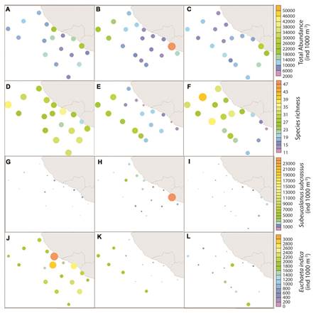
Fig. 4 Monthly total abundance (A-C), species richness (D-F), Subeucalanus subcrassus abundance (G-I) and Euchaeta indica abundance (J-L). Months are January (Jan) (A, D, G, J); May-June (May) (B, E, H, K) and October (Oct) (C, F, I, L). Note the different color scales for each variable.
Copepod distribution and species groups: The CA indicated that there were four principal assemblages present across the surveyed periods (Fig. 5A). The Jan EN cluster (G1) was comprised of nearly all the stations sampled in Jan. There was a small sub-cluster, which included the coastal stations in this group, but otherwise there was no relevant grouping pattern. The May offshore cluster (G2) was totally comprised of stations from the May survey period located 100 nm from the coast, but did not include the stations closest to the cyclonic eddy. The Oct LN cluster (G3) was principally comprised of stations from the Oct survey period. The May coastal and eddy upwelling cluster (G4) was composed of May stations affected by coastal upwelling or associated with the cold-core cyclonic eddy, but also included stations from Oct which were located in areas of coastal upwelling and the small cyclonic eddy in the Southern region during that period. The MRPP confirmed that the groups defined by the CA were significantly different (P < 0.05). ANOVA indicated that there were no significant differences in total abundance across the cluster groups (P > 0.05), but species richness and diversity were significantly lower in May upwelling than all other groups (P < 0.05). SIMPER analysis showed that Eucalanidae and Euchaetidae were the most abundant families, with copepodites contributing the most abundance all four of the cluster groups (Table 3). However, the relative abundance varied between periods. Adults and copepodites of Euchaetidae contributed the highest percentage of abundance to the relatively more diverse Jan EN (26.76 %) and May offshore (21.21 %) clusters, while adults and copepodites of Eucalanidae contributed the highest abundance to the Oct LN (25.91 %) and May upwelling (41.83 %) clusters. Copepodites of Euchaetidae dropped to their lowest relative contribution during May upwelling. The IVA resulted in 9 significant indicators for Jan EN, 8 for May offshore, 3 for Oct LN, and only 1 for May upwelling (Table 4). Pontellina sobrina had the highest percentage IVA of all species, with 65.3 for Jan EN, followed by Paraucalanus sewelli with 59.3 for May offshore.
Table 3 SIMPER analysis % contribution of species/families contributing to 90 % abundance of the groups defined by the cluster analisis
| Group | Average Similarity | # spp | Species (% Contribution abundance) 1 |
|---|---|---|---|
| G1: Jan (El Niño) | 62.47 | 32 | EhJu (12.55), Ein (8.14), EucJu (7.00), Onc (4.09), CalJu (3.98), Cpau (3.73), Ssut (3.44), Er (3.42), Sc (3.36), Clm(3.31), MeJu (3.17), Pj (2.83), Ssu (2.70), El (2.65), Al (2.30), Sma (2.10), Cm (2.07), Ctr (1.84), Sb (1.80), ScJu (1.76), Pso (1.66), ClJ (1.63), Ag (1.49), AtJu (1.48), Cd (1.33), Uv (1.33), CanJu (1.16), Os (1.08), Ab (0.97), Scr (0.82), Ppi (0.80), Td (0.74) |
| G2: May Offshore | 67.41 | 25 | EhJu (11.33), Ssut (7.98), EucJu (6.93), Cd (5.95), Ein (5.81), CalJu (4.67), Mt (4.58), El (4.07), (3.97), Sb(3.63), (3.45), Sd (3.40), Pj (3.00), MeJu (2.81), Ps (2.68), Ctr (2.39), Scu (2.30), Sm (2.03), Ssu (1.64), Nm (1.61), Scr (1.43), Ab (1.37), Td (1.33), AtJu (1.28), Pg (1.16) |
| G3: October (La Niña) | 61.53 | 25 | EucJu (14.12), EhJu (7.22), Ssu (5.32), CalJu (5.19), Sb (4.91), Ssut (4.59), Cpau (4.44), MeJu (4.07), Td (3.92), Nm (3.44), El (3.11), Al (2.90), Ab (2.46), ScJu (2.25), Sa (2.23), Acr (2.19), Cf (2.13), Ein (1.88), AtJu (1.68), Pj (1.52), Sc (1.48), Uv (1.48), Mt (1.39), Coc (1.33), Aa (1.29), TeJu (1.27), PoJu (1.23), Ppi (1.14) |
| G4: May Eddy and Coast upwelling | 60.48 | 18 | EucJu (21.12), SSu (17.57), Cf (7.01), Td (6.97), MeJu (5.27), Sb (5.02), TeJu (4.60), Ssut (3.14), Ab (3.10), Sc (2.89), Scr (2.51), Pj (1.79), Cpau (1.78), Sa (1.78), AtJu (1.75), EhJu (1.68), Nm (1.66), El (1.57) |
1Aa = Acrocalanus andersoni, Ag = A. gracilis, Al = A. longicornis, Ab = Aetideus bradyi, AtJu = Aetideidae copepodites, CalJu = Calanidae copepodites, CanJu = Candaciidae copepodites, Cd = Cosmocalanus darwini, Cf = Centropages furcatus, Clj = Clausocalanus jobei, Clm = C. minor, Cm = Calanopia minor, Coc = Corycaeus crassiusculus, Cpau = Canthocalanus pauper, Ctr = Candacia truncata, Ein = Euchaeta indica, El = E. longicornis, Er = E. rimana, EhJu = Euchaetidae copepodites, EucJu = Eucalanidae copepodites, MeJu = Metridinidae copepodites, Mt = Mesocalanus tenuicornis, Nm = Nannocalanus minor, Onc = Oncaeidae spp, Os = Oithona setigera, Pg = Pleuromamma gracilis, Pj = P. johnsoni, Ppi = P. piseki, PoJu = Pontellidae copepodites, Ps= Pareucalanus sewelli, Pso = Pontellina sobrina, Sa = Scolecithricella abyssalis, Sb = Scolecithrix bradyi, Sc = Scolecitrichopsis ctenopus, ScJu = Scolecitrichidae copepodites, Sd = Scolecithrix danae, Sm = Sapphirina metallina, Sma = Scolecithricella marginata, Scr = Subeucalanus crassus, Ssu = S. subcrassus, Ssut = S. subtenuis, Td = Temora discaudata, TeJu = Temoridae copepodites, Uv = Undinula vulgaris
Table 4 Species and copepodite taxa with significant indicator values for each cluster group
| Cluster / Group | Taxa | IV 1 | Mean | (SD 2 ) | p |
|---|---|---|---|---|---|
| G1: Jan (El Niño) | Pontellina sobrina | 65.3 | 21.2 | (6.33) | < 0.001 |
| - | Clausocalanus jobei | 58.2 | 21.8 | (5.96) | < 0.001 |
| - | Clausocalanus furcatus | 57.9 | 16.5 | (6.79) | 0.001 |
| - | Paracalanus aculeatus | 49.5 | 17.5 | (6.80) | 0.002 |
| - | Acrocalanus gracilis | 46.8 | 22.7 | (5.91) | 0.003 |
| - | Candaciidae copepodites | 40.1 | 24.1 | (5.37) | 0.012 |
| - | Lucicutia gaussae | 38.8 | 19.6 | (6.24) | 0.009 |
| - | Paracalanidae copepodites | 36.9 | 17.8 | (6.66) | 0.027 |
| - | Acartia negligens | 28.6 | 11.4 | (6.29) | 0.017 |
| G2: May Offshore | Pareucalanus sewelli | 59.3 | 20.5 | (6.62) | < 0.001 |
| - | Pleuromamma gracilis | 56.6 | 14.9 | (6.90) | < 0.001 |
| - | Scolecithrix danae | 55.9 | 22.4 | (5.97) | < 0.001 |
| - | Centropages gracilis | 47.5 | 16.8 | (6.63) | 0.002 |
| - | Corycaeus robustus | 38.7 | 14.8 | (6.95) | 0.005 |
| - | Corycaeus speciosus | 38.4 | 20.7 | (6.30) | 0.015 |
| - | Aetideus armatus | 35.9 | 19.8 | (6.56) | 0.030 |
| - | Lucicutia flavicornis | 29.2 | 16.8 | (6.64) | 0.047 |
| G3: October (La Niña) | Eucalanus inermis | 43.4 | 14.8 | (6.86) | 0.006 |
| - | Corycaeus crassiusculus | 38.8 | 22.2 | (5.91) | 0.025 |
| - | Rhincalanus nasutus | 35.7 | 10.9 | (6.13) | 0.006 |
| G4: May Eddy and Coast upwelling | Rhincalanus rostrifrons | 21.4 | 9.4 | (5.49) | 0.047 |
IV = Indicator value.
SD= Standard deviation.
Association with environmental variables: The seasonal and interannual distribution of environmental variables and their effect on the copepod community were analyzed using CCA, with stations labeled a priori as inshore/offshore and by month, with CA groups shown as dotted lines connecting the stations (Fig. 5B). The MRPP confirmed that the inshore/offshore groups were significantly different (P < 0.05). The first two axes explained 21.5 % of the variance seen in species data, with a Pearson Species-Environment Correlation of 0.930. Axis 1 explained the greatest amount of variation, primarily through surface (0-50 m) temperature, salinity, phosphorus, nitrates+nitrites, and sub-surface (75-200 m) ammonium. Axis 2 was most closely associated with dissolved oxygen. The CCA biplot showed that the groups had a well-defined distribution associated with environmental conditions, although with the presence of some slight overlap (Fig. 4A). Stations from the G4 upwelling cluster were distributed along the upper right side of the graph, showing correlations with lower surface temperature, higher surface nitrites+nitrates and salinity, indicative of upwelling conditions. G3 Oct LN stations were primarily grouped in the center of the biplot, showing the modification of what is usually the warmest and least productive period in the region to slightly cooler, more productive conditions in the water column. The G2 May offshore stations did not show a high association with the environmental variables, indicating that other processes affected the species composition of those groups. G1 EN cluster stations were primarily associated with high temperatures and subsurface ammonium.
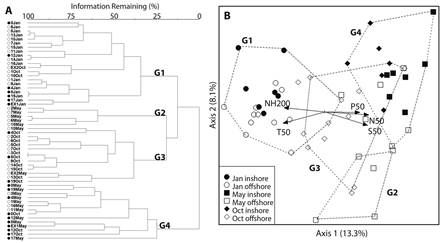
Fig. 5 A. Cluster analysis dendrogram of sample sites resulting in 4 groups: G1= Jan EN cluster; G2 = May offshore cluster; G3 = Oct LN cluster; G4 = May coastal and eddy upwelling cluster. Filled symbols are inshore sites, open symbols are offshore sites. B. Canonical Correspondence Analysis biplot of sample sites and environmental variables; sample symbols were defined a priori as inshore and offshore sites by month. Sample groupings (dotted lines) are results of cluster analysis. Environmental variables (arrows) in multivariate space with > 0.400 r2 value are shown: T50 = 0-50 mean temperature (°C); NH200 = mean 75-200 m ammonium (µM); S50 = 0-50 m mean salinity; N50 = 0-50 m mean nitrate+nitrite (µM); P50 = 0-50 mean phosphorus (µM).
Discussion
Tropical copepods form a large part of zooplankton biomass and are therefore important drivers of zooplankton productivity, but the impact of physical and biological variables on copepod community structure is poorly known in the ETPM. The analysis of the effect of hydrological changes such as increased temperature on species distribution and abundance can provide a baseline to understand the effects of short-term variability such as ENSO and long-term hydrological modifications driven by climate change on copepod community structure. The present study includes three seasonally distinct survey periods -Jan (transitional), May (tropical CC and coastal upwelling), and Oct (MCC and coastal downwelling) that were also distinguished by EN (Jan), ENSO neutral (May) and LN (Oct) conditions- over the course of one year. We found that during the EN sampling period, the structure and abundance of the copepod community was affected by the modification of regional hydrodynamics, enhancing the intrusion of carnivorous species and causing a decrease in total abundance which was maintained throughout the ENSO neutral and Oct LN periods.
The contrasting effects of EN and LN on temperature and water column stability appeared to modify the established pattern of currents and coastal upwelling during the study period, processes which have been reported to have strong effects on zooplankton and ichthyoplankton communities in both oceanic and coastal regions of the ETPM (Ambriz-Arreola, Gómez-Gutiérrez, Franco-Gordo, Lavaniegos, & Godínez-Domínguez 2012; León-Chávez, Beier, Sánchez-Velasco, Barton, & Godínez, 2015). Portela et al. (2016) discussed water masses and circulation in the central Mexican Pacific; the geostrophic flows reported in their study varied from those seen in 2010, probably due to the El Niño (Jan) bringing TSW across the entire region and La Niña (Oct) disrupting the northward flowing MCC and inducing an anomalous intrusion of sub-surface CC water -the oceanic, tropical extension of this current is usually strongest in spring (Kessler, 2006). Two specimens of Calanus pacificus, a species of temperate affinity (Palomares et al., 1998), were recorded in the Northern offshore transect during Oct 2010, corroborating our reported intrusion of CCW. To the best of our knowledge, this is the first report of this CC species indicator, which has been reported along the Baja California Peninsula and the Gulf of California, in the central Mexican Pacific (Brinton, Fleminger, & Siegel-Causey, 1986; JiménezPérez & Lavaniegos, 2004). Although LópezIbarra et al. (2014) only included species with abundances > 80 % in their study along the entire Mexican Pacific, and it is possible that some few unreported specimens were also present further South. Based on historical CUI values and on López-Sandoval et al. (2009), coastal upwelling and primary productivity, coastal upwelling is usually low in Jan (transitional), relatively high in May, and relatively low to absent in Oct. This pattern was apparently modified by both EN and LN, as Chl a concentrations were very high in Jan (EN), and the CUI was positive for Oct (82.4), with patches of relatively cool surface waters due to extensive coastal upwelling and a small cyclonic eddy to the south, probably resulting from the thermocline-lifting effect of the LN. Kurczyn et al. (2012) characterized mesoscale activity in this region (Cabo Corrientes in that study, corresponding to the ETPM) and found relatively high levels of both anticyclonic and cyclonic eddies, which were associated with seasonal peaks in currents and CUI and no statistically significant association with EN events. Due to the short duration of the present study, it is not possible to confirm a definite effect of EN on eddy production; however, considering that both coastal upwelling events and current processes were modified, it is very possible that an effect occurred on eddy generation, subsequently affecting the ecology of the study area.
There were no significant differences in copepod abundances between the survey periods of the present study. Kozak et al. (2014) studied adult calanoid copepods from the inshore region of the present study area (19° N, 104° W), using the same methodology (oblique hauls using a 505 µm mesh net), and reported abundances between 50-200 ind./m3 per month, with the lowest values in the EN and post EN periods. In the present study, the inshore abundances of adult calanoid copepods per month averaged 7.2 ind./m3 (Jan), 7.7 ind./m3 (May) and 4.4 ind./m3 (Oct), with a maximum value of 34.3 ind./m3 during May (station 17). Therefore, we hypothesize that the lack of significant differences in abundance between the three periods resulted from the EN event at the start of our study period, which depressed this larger size fraction of copepod abundance through at least Oct. Jiménez-Pérez (2016) also reported significantly lower copepod abundances during EN in Bahía de Banderas (Nayarit, Mexico), demonstrating that this is a region-wide response to EN events. There is still a much uncertainty regarding the impact of climate change on ENSO (Collins et al., 2010). However, this study indicates that if EN anomalies increase in frequency and/or strength due to global climate change, the rapid succession of disturbances without a sufficient recovery period could have marked repercussions in the overall zooplankton abundance and community resilience, impacting marine ecosystem productivity.
The species composition in this study is very similar to that reported in Kozak et al. (2014); there were no significant alterations in species composition between surveys and most of the same species were present across the different hydrological periods. However, the relative abundances of species did vary between surveys in both studies. During the Jan EN period of this survey, the influx of TSW across the entire studied region induced high species diversity and no inshore-offshore gradients of abundance, S or H’. Oct (LN period), which usually presents uniformly warm temperatures across the region due to the influence of the MCC and relatively high inshore species diversity (Kozak et al. 2014), showed comparatively low S and H’. During May, which was ENSO neutral, a cyclonic mesoscale eddy, coastal upwelling, and an inshore-offshore temperature gradient were re-established, along with lower values of S and H’. Recent studies in the ETPM have shown the important effects of mesoscale processes (upwelling, eddies) on zooplankton distribution and structure (LeónChávez, et al., 2010; Davies et al., 2015). Cruz-Hernández et al. (2018) reported a significant vertical stratification of calanoid copepod species in a mature cyclonic eddy in the Gulf of California, and found that herbivorous/ omnivorous species were dominant. We did not find significant correlations with total abundance, however, species richness in the May upwelling cluster (cyclonic eddy and coastal stations) was significantly lower than all other cluster-defined groups (P < 0.05) with larger, generally herbivorous copepodites of Eucalanidae and Subeucalanus subcrassus dominating the assemblage. Even though the abundances of adults and copepodites of Euchaetidae were low in the upwelling assemblage, in the May offshore assemblage they maintained high levels. Eucalanidae (primarily Subeucalanus subcrassus) may dominate during the more productive periods, but Euchaetidae appears to maintain high abundance values of adults and copepodites in the warm offshore regions that are not affected by cyclonic eddies and which can invade the coast rapidly when conditions permit. This appears to have occurred in Jan, when there was no upwelling grouping despite what appeared to be a mature cyclonic eddy in the oceanic region; the EN appeared to homogenize the offshore/inshore/eddy species distribution and the relatively high temperatures precipitated dominance of Euchaetidae.
Despite upwelling events in May and Oct with high nutrient values and low temperatures that should correlate with high primary productivity, 0-50 m Chl a values were highest in Jan, especially in one coastal station and in the weak cyclonic eddy. High ammonium values could be from increased zooplankton metabolism (due to high temperatures) or microbial loop activity, both of which primarily excrete nitrogen as ammonium (Corner & Newell, 1967). This could have provided some of the nutrients required for the observed high phytoplankton production (Alcaraz, Saiz, & Estrada, 1994). Pelayo-Martínez et al. (2017) hypothesize that the values seen in this same study period could be due to removal of the top down control by herbivorous zooplankters on phytoplankton growth by carnivorous zooplankters. Our study aligns with these hypotheses, as we found that oceanic, carnivorous copepod species (primarily Euchaeta adults and Euchaetidae copepodites) were most abundant during the Jan EN period across the entire region. This also has important implications for the trophic structure of the region. Due to the relatively small size of these organisms in comparison to other carnivorous zooplankters (e.g. chaetognaths), they prey on much smaller organisms, probably eggs and early larval stages of planktonic organisms. Therefore, the transfer of carbon biomass could be reduced, as well as the overall productivity of the ecosystem. In addition, as warming trends continue, not only can tropical copepod size be reduced due to increased metabolism, but there could be a regime shift to smaller species. A “tropicalization” of the copepod community during the 1997/98 EN was reported off the coast of Baja California by Jiménez-Pérez and Lavaniegos (2004), and it is generally accepted that continued warming events will contribute to that anomaly, with smaller tropical copepod species expanding their distribution into more temperate regions. However, the indicator species assemblage (highest percentage IVA) for the Jan EN period was primarily composed of relatively smaller (< 1 100 µm) species than most of the May and October surveys significant indicators (> 1 500 µm). This suggests that even what has been a fairly stable tropical assemblage is not immune to the biogeographic redistribution of species that has been observed in higher latitudes (Beaugrand, Reid, Ibanez, Lindley, & Edwards, 2002).
This study was limited by the short sampling duration (< 1 year) that did not include non-anomalous seasons for comparison. In addition, there were certainly species (especially cyclopoid copepods) that were undersampled due to the relatively large-sized mesh (505 µm) of the sampling net. A smaller mesh size would have been ideal for a more complete analysis of the copepod community. Regardless, the results of this study are still valuable due to the proportionally high abundance of these larger copepods in this marine ecosystem; Pelayo-Martínez et al. (2017) reported that the copepods from this study accounted for 71 % of total zooplankton abundance. As the dominant organisms in this larger size fraction, they play an important role in overall zooplankton productivity and trophic dynamics, and variations in their abundance could have a large impact on the ecology of the region.
In summary, the species distribution of copepods in the central Mexican Pacific appears to be principally defined by seasonal modifications of the water column as well as mesoscale eddy processes in the oceanic region and by upwelling episodes in the inshore region. The mesoscale processes are affected by ENSO events, which in the case of EN seem to disrupt the inshore -offshore gradient, import carnivorous, offshore species into the inshore area, cause marked reductions in copepod abundance across the entire ETPM, and increase dominance of smaller sized species. Future studies in the region should incorporate smaller mesh sized nets, stratified samples, and a longer time series to study three-dimensional variability of copepods in a transitional oceanographic region that is markedly affected by interannual anomalies.

