


Services on Demand
Journal
Article
 Article in xml format
 Article references
 Send this article by e-mail
Indicators
-
 Cited by SciELO
 -
 Access statistics
Related links
-
 Similars in
SciELO
Similars in
SciELO  uBio
uBio
Share

 Permalink
Revista de Biología Tropical
On-line version ISSN 0034-7744Print version ISSN 0034-7744
Rev. biol. trop vol.52 suppl.2 San José Dec. 2004
Bay, Gulf of Papagayo, Pacific coast of Costa Rica and its value
as bioindicator of pollution
Melinda Bednarski1* & Alvaro Morales-Ramírez2
1 Center for Tropical Marine Ecology (ZMT), Fahrenheitstrasse 6, D-28359 Bremen, Germany.
2 Centro de Investigación en Ciencias del Mar y Limnología (CIMAR) y Escuela de Biología, Universidad de Costa Rica, 2060, San Pedro, Costa Rica; amorales@cariari.ucr.ac.cr
* Corresponding Author: Marine Invasions Research Laboratory, Smithsonian Environmental Research Center, 647 Contees Wharf Road, Edgewater, Maryland 21037, USA; bednarskim@si.edu
Received 13-XI-2003. Corrected 25-II-2004. Accepted 13-IV-2004.
Abstract
The abundance, distribution and composition of the macrozooplankton of Culebra Bay, Costa Rica (10º 38 N - 85º 40 W) were studied at four stations throughout the dry (February - May) and rainy (September - November) seasons of 2000. The samples were collected at two-week intervals using a 500µm mesh net with a 0.5 m diameter opening. Copepods (23-31%) and ostracods (20-34%) were predominant throughout the year, followed by cladocerans (2.5-14%), zoea (6.6-9.5%), and siphonophores (2.5-7.2%). High densities of zooplankton were obtained in February and March with peak abundance on March 18. The lowest densities were observed on September 3 and November 5. Significant differences in abundances at each station were observed for the groups Acartia tonsa (Copepoda), Ctenophora, Medusae, Ostracoda, Zoea, and Amphipoda. Comparison of the dry and rainy seasons revealed significantly higher zooplankton abundance in the dry season and copepod domination of all stations; during the rainy season ostracods dominated the off-shore areas. Zooplankton abundance and distribution are influenced by upwelling, which occurs during the dry season in Culebra Bay.
Key words: macrozooplankton, pollution, Eastern Pacific, MDS, microcrustacean, Culebra bay, Costa Rica.
The study of marine ecosystems is important since human activities play an increasing role in altering these areas. Through these studies there is a growing awareness of the importance of zooplankton, which has been found to be the primary food source for more than fifty percent of fish species and their larval stages. Pelagic zooplankton also plays an extremely important role in the transfer of organic material from primary producers to predators via the food web. For this reason one of the determining factors of commercial fisheries is the production of pelagic zooplankton, the population fluctuations and composition of which directly affects their predators (Cushing, 1995). Recent studies have confirmed that through the food chain toxins and other compounds from dinoflagellates can be passed onto herbivorous zooplankton and then accumulate in zooplanktivorous fish. In these studies fish were not directly exposed to the toxins, but instead accumulated them by feeding upon copepods that had grazed on the dinoflagellates (Tester et al. 2000). The sinking of detrital material from zooplankton populations via fecal pellets, moults, and carcasses, represents an important mechanism for rapidly transferring compounds from upper to deeper parts of water bodies. Within zooplankton, copepods are usually the dominant group in terms of biomass and are of key importance in the transfer of compounds from the environment via phytoplankton to zooplanktivorous fish and then on to top predators – including humans (Hopcroft and Roff, 1998).
Zooplankton organisms are considered to be the ecological indicators or bioindicators of water bodies. They can provide information on trends in environmental conditions and how these conditions affect the indicator itself (Vandermeulen, 1998). Bioindicators are increasingly being used in fields such as Coastal Zone Management as viable ways to monitor the sustainability and health of ecosystems. They are used to indicate contaminant exposure, to provide early warning of impending environmental damage, to link causes of stressors to ecologically relevant effects, and in ecological risk assessments (Bioindicators, 1999).
The distribution and abundance of bioindicators in polluted and unpolluted waters can provide useful information on the health of their habitat. The stability of the environment is dependent on external stress. A stable environment can sustain a diversified faunal assemblage, which is indicative of healthy conditions. A growing number of studies in the tropics have utilized coastal zooplankton communities for water quality assessment and as indices of eutrophication. Pelagic communities that are stressed have reduced species diversity, and population sizes of some species are greatly increased which causes periodic pulses in the zooplankton community (Lindo, 1991).
An increase in organic pollution along coastlines is correlated with higher rates of phytoplankton production, which leads to zooplankton communities of higher biomass. Recent investigations have lead to the creation of zooplankton indices that can be used to monitor eutrophication (Bioindicators, 1999). Some copepod species tend to cluster in a facies manner around polluted sites. The areas closest to the pollution source having the lowest species diversity with the present few species being tolerant of conditions such as oxygen deficiency, enhanced nutrient levels, and increased turbidity. Several ecological assessments have found that the input of a pollutant can cause the entire species hierarchy to be metamorphosed. Further away from the source more species are found until an area is reached where the community is considered to have "normal" structure in terms of diversity and abundance (Arfi et al. 1981).
Many studies have shown that the abundance of zooplankton varies seasonally as well as with physical changes in the environment (Reeve, 1970, Haridas et al. 1980, Youngbluth, 1980, Diaz-Zaballa and Gaudy, 1996). In a two year long study Youngbluth (1980) worked in a tropical embayment of Puerto Rico where he determined that the limited circulation of the bay influenced the location where certain zooplankton species were found in the bay and the abundance of these species. The lowest number of species occurred farthest within the bay and the greatest number at the mouth of the bay. The largest changes in zooplankton abundance occurred during the rainy season with copepod biomass two to three times greater than during the dry season. In the areas of highest zooplankton density the copepod species Acartia tonsa formed between fifty and ninety percent of the zooplankton community. Díaz-Zabella and Gaudy (1996) found in a study of a eutrophic bay in Cuba that zooplankton abundance corresponded to fluctuations of abiotic factors like salinity and temperature due to the occasional flushing of the bay rather than to phytoplankton abundance. The abundance of total zooplankton was highest during the summer months when the water salinity and temperatures were at minimum levels. Zooplankton abundance was correlated more to salinity levels than to temperature. The rotifer Brachionus plicatilis appeared only in the summer months during the lowest salinity measurements. The abundance of copepod eggs and of successive copepodites was not dependent on environmental factors like temperature, salinity, or chlorophyll but on the number of adult males or females. The temperature and salinity fluctuations and not the phytoplankton cycle were believed to be the cause of the sex ratio variation found in copepod species Acartia tonsa. It was observed that males were more sensitive to the hydrology changes, diminishing at a greater proportion when the whole population decreased (Díaz-Zabella and Gaudy, 1996).
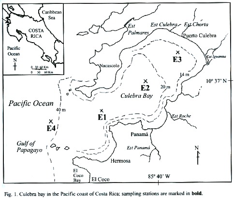
The present study took place in Culebra Bay, within the Gulf of Papagayo on the northern Pacific coast of Costa Rica (Fig. 1). It is an area of intense outcrops, rugged terrain, and increasing coastal development (Jiménez, 2001). Our goals were to contribute to the knowledge of macrozooplankton biodiversity of the Pacific coast of Costa Rica, analyse time series data in order to better understand the macrozooplankton population dynamics in Culebra Bay, and relate the variance in abundance composition of macrozooplankton to the physical and chemical (salinity, temperature, oxygen concentration, and turbidity) conditions in Culebra Bay with special reference to copepods.
Materials and methods
Description of study site: The Gulf of Papagayo is located on the northern Pacific side of Costa Rica (Fig. 1). It encompasses Culebra Bay, whith species (sea turtles, rays, and dolphins) common to the Pacific. Culebra Bay has coral reefs making it attractive for sport diving and as a tourist destination (Jiménez, 1998). The area of Culebra Bay has been designated by the Costa Rican government for prime tourist development within the next 10 years (Papagayo, 1999). The climate of Culebra Bay is influenced by seasonal displacements of the tropical convergence zone (ITCZ) and the intensification of the NE tradewinds, which define the dry (December-April) and rainy (May-November) seasons. During the dry season the trade winds instigate upwelling bringing cooler nutrient-rich water from the water depths to the surface where marine life thrives (Gross, 1993). The ocean currents of the Pacific side of Central America are characterized by a strong westward surface North Equatorial Current at about 1° N, a weak eastward Counter Current at 5º N, and the westward Equatorial current at the equator that extends to 5° S (Fujita and Fujuita, 1998). The currents near Costa Rica are heavily influenced by the transition between the northeast and southeast trade winds, which are in a transitional state in this area. The area of this transition is known as the Intertropical Convergence Zone (ITCZ) and lands within this area are characterized by strong seasonal changes of dry summers (December-April) and high amounts of rainfall in the winter (May-November). The Costa Rica coastal current runs northward along the Pacific Coast and is the primary current affecting the Culebra Bay area for most of the year. The coastal currents are influenced by the intensity and direction of the tides, which are relative to the seasonal and local variations produced in the estuary system within the bay (Wallace and Hobbs, 1977). Generally, within Culebra Bay the waters are believed to flow in from the south, around the bay, and back out through the northern lip of the mouth.The area of Culebra Bay is characterized by reef outcrops around the mouth of the bay and at a few areas within the bay intermingled with sandy beaches. Amangrove estuary is located in the northeast part of the bay (Estero Iguanita, Fig. 1) and two smaller estuaries also fringe the inner bay. The land surrounding the bay is rugged and the vegetation of the type that can withstand long dry spells (Glynn et al. 1983).
Tourism is a growing influence in the Gulf of Papagayo, Culebra Bay area. The Papagayo Tourism Project was initiated in 1972 to develop the area into an international tourist pole, which is hoped to become the main tourist destination of Costa Rica. The influence of this project can be seen in the numerous hotels recently constructed in the area, the many activities geared for tourists like diving safaris and sport fishing, and the growth of El Coco a small city just south of Culebra Bay.
Sampling: Four stations were located from offshore to near-shore in Culebra Bay (Fig. 1): Station 4 (E4) farthest offshore, outside bay mouth (40 m deep); E1 in the bay mouth (20m deep); E2 mid-bay (20m deep); and E3 near-shore (14-15 m deep).
Data was collected during the rainy and dry seasons from September 2000 to February 2001. Sampling occurred in two-week intervals with every station being sampled on the same day. Sampling took place early in the day between 06:00-13:00 and the stations were always visited in the same order (E4, E1, E2, then E3). The four sampling stations followed previous and ongoing studies (Rodriguez, unpublished; and Morales-Ramirez, study in progress). The stations were reached by boat and positions were checked using a GPS unit.
At each station the weather conditionswere noted and water samples collected with a Niskin oceanographic bottle in five-meter depth increments at E4, E1, and E2, and at three-meter increments at the shallowest station, E3. The water was used for analyses of temperature, salinity, and dissolved oxygen. The temperature recordings were used to determine whether or not there was a thermocline in the water column. If a thermocline was determined to be present two vertical net tows were collected using the Nansen system: one from the deepest depth to below the thermocline and the second from the thermocline to the water surface - otherwise, a single tow of the water column was done. A Secchi disc was used to measure the turbidity of the water.
Plankton sampling at each station wasdone as described in von Wangelin and Wolff (1996) using a 500-micron net with opening diameter 50 cm. The net was washed with seawater to collect the plankton into a jar. All samples were dated and recorded in a log-book. The plankton were fixed with 4% formalin and then taken to the CIMAR laboratories for analyses.
Processing of Samples: Fractionation, identification and enumeration. Following Alvariño (1981) samples were fractionated to the desired level. Main groups of zooplankton were identified to Order and counted. Copepods were identified to the most specific level possible. The numbers of organisms in each fraction were converted to densities, number of individuals m-3 . Comparisons were made of the numbers of organisms at different stations, the total numbers during dry versus rainy seasons, the difference in water chemical data between stations and seasons, and specifically, the difference in densities between copepod species.
A sample/species matrix of abundance data was constructed for PRIMER 5 with factors of season, date, station (distance), and whether the sample was taken above the thermocline, below, or of the entire water column. Two main matrices were used – one with all the samples and a second in which samples were combined into a complete water column. Samples had labels of A through H with corresponding numbers in order of sampling dates. For example for the total water column analysis, E4 dry season samples had identifiers of A1 – A7 and E4 rainy season samples had identifiers of B1 - B5. In this method E1 samples had identifiers beginning with letters C and D, E2 of letters E and F, and E3 of letters G and H. Abiotic environmental data of oxygen content, salinity, temperature, and turbidity were also considered. Multi-Dimensional Scaling, Cluster, Species contributions to similarity and Biota and/or Environment matching analyses were performed and species area curves were constructed following statistical references and the PRIMER 5 handbook (Clarke and Gorley, 2001, Borg and Groenen, 1997, and Clarke and Warwick, 1994).
Results
Overview of hydrology: The oxygen, salinity, temperature and Secchi measurements made simultaneously with the zooplankton samplings of Culebra Bay during the dry and rainy seasons are shown in Fig. 2. The dry season was sampled from 5 February through 20 May. The rainy season was sampled from 3 September until 19 November. Missing values resulted from a malfunctioning water quality meter on 26 February and 6 May.
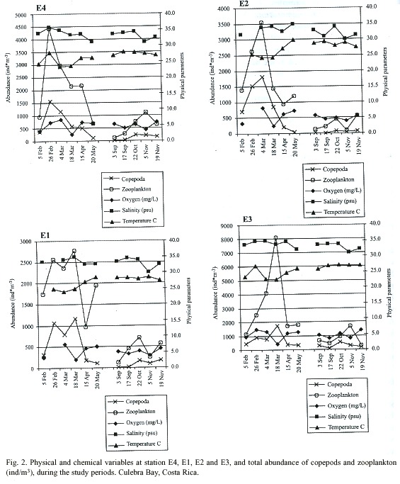
Oxygen measurements were more dynamic during the dry season than in the rainy season. Readings in the dry season ranged between 0.4 and 9.6 mg/L versus between 1.4 and 8.1 mg/L during the rainy season. During the dry season minimum values occurred on 18 March at all stations with averaged water column oxygen readings between 1.8 (E4) and 2.5 mg/L (E2). Minimum oxygen measurements during the rainy season occurred on 5 November with averaged water column readings between 3.4 (E1) and 3.9 mg/L (E3). Maximum averaged water column oxygen readings occurred on 4 March during the dry season at stations E1 (6.8 mg/L), E2 (7.5 mg/L), and E3 (8.2 mg/L). E4 averaged 5.8 mg/L on this date and was maximum on 26 February with 6.6 mg/L. During the rainy season maximum averaged water column oxygen readings occurred on 19 November at stations E4 (6.2 mg/L), E1 (5.8 mg/L), and E2 (5.9 mg/L). E3 averaged 5.6 mg/L on this date and was maximum on 3 September with 5.7 mg/L.
Salinity readings on average were higher during the dry season than in the rainy season. Readings taken during the dry season varied between 30-36 and between 30-35 during the rainy season. Low average water column salinity of 31 was recorded on 20 May at E1. On this date salinity averaged 32 at E4, 33 at E2, and 35 at E3. On 5 February a low average water column reading of 32 was recorded at E3. On this date salinity averaged 34 at E4 and E1, and 33 at E2. Minimum salinity readings during the rainy season were taken on 5 November with average water column measurements of 31 at E4 and E1 and 30 at E2 and E3. Maximum salinity readings during the dry season were recorded on 26 February with average water column readings at E4 of 35, and of 36 at E1. Further data for this date is unavailable due to mechanical failure of the water quality meter. During the rainy season the maximum values occurred on 22 October at an average of 34 at stations E4, E1, and E3. E2 also averaged 34 on this date but had a maximum average on 17 September of 35.
Temperature readings ranged between 19 and 30°C during the dry season and between 22.5 and 3ºC during the rainy season. Minimum readings were recorded for the dry season during March. On 5 March water column averages were lowest for E1, E2 and E3 with 23.5, 24.0 and 24.2ºC respectively. E4 had an average reading of 22.7ºC. On 18 March E4 had an average reading of 22.6ºC and E1, E2 and E3 measured 23.7, 24.9, and 24.3ºC respectively. During the dry season minimum averaged water column temperature readings occurred on 19 November at all stations: E4, 26.8ºC; E1, 26.9ºC; E2, 27.5ºC; and at E3, 27.6ºC. Maximum temperature readings during the dry season were recorded on 26 February with an average water column temperature at E4 of 26.0ºC, and of 27.8ºC at E1. Further data for this date is unavailable due to mechanical failure of the water quality meter. Maximum temperature readings during the rainy season were recorded on 17 September for stations E4 (26.9ºC), E1 (27.9ºC), and E3 (29.4ºC). E2 averaged 28.3ºC on this day and had a higher average of 28.5ºC on 5 November.
Thermoclines were determined to be present during the dry season at E4 on 5 and 26 February at 20 meters depth from the surface, on 18 March and 15 April at 15 meters, and on 20 May at 25 meters. During the rainy season thermoclines at E4 were determined to be present on 3 September at 15 meters, on 17 September and 5 November at 35 meters, and on 22 October at 20 meters. At E1 thermoclines were determined to be present during the dry season on 26 February and 15 April at a depth from the surface of 15 meters, and on 20 May at 10 meters. In the rainy season thermoclines were present at E1 on 3 September at 15 meters, on 17 September at 20 meters, and on 5 November at 25 meters. A thermocline was determined to be present at E2 only in the dry season on 20 May 15 meters from the water surface. No thermoclines were found in the dry or the rainy season at E3.
The highest turbidity measurement of the dry season was recorded at E3 on 20 May with depth of 3.2 meters. On this date all other stations recorded lowest turbidity measurements. Highest turbidity for E4 and E1 occurred in March with 4.7 meters on both sampling dates. Highest turbidity at E2 occurred on 5 February with 5.1 meters. During the rainy season measurements of highest turbidity occurred on 17 September for all stations ranging between 4 meters at E3 and 7.4 meters at E4. Lowest turbidity occurred on 5 November for all stations with Secchi measurements ranging between 11.0 meters at E3 to 15.7 meters at E1.
BIOENV best results in PRIMER revealed that salinity was correlated to temperature (0.282), turbidity (0.203) and oxygen (0.113); oxygen was correlated to temperature (0.228); and temperature correlated to salinity and turbidity (0.223). Turbidity was correlated to all the variables by 0.164.
The correlation matrix was used to identify additional significant relationships between the variables of season, station, depth of sample, salinity, oxygen, temperature, and turbidity. The Pearson coefficient, r, was used to identify to which extent the values of two variables were "proportional" to each other. Correlations were significant at p < 0.5000. In relation to season, temperature (r = 0.374, p = 0.004) and turbidity (r = 0.546, p = 9.49E-06) measurements were significantly proportional. The depth of the station had an effect on salinity (r = 0.263, p = 0.457), temperature (r = -0.375, p = 0.004), and turbidity (r = 0.332, p = 0.011). Salinity measurements were proportional to temperature (r = 0.263, p = 0.0004) as were those of oxygen (r = 0.466, p = 0.0002).
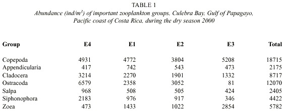
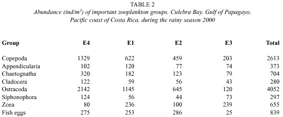
Zooplankton: Sixteen groups were identified in the sixty-six samples: Appendicularia, Chaetognatha, Cladocera, Copepoda, Ctenophora, Euphausiacea, Medusae, Ostracoda, Polychaeta, Salpa, Siphonophora, zoea, Amphipoda, Branchiopoda, Gastropoda, Stomatopoda. Abundances of fish larvae, vertebrate eggs, barnacle naupliae, crustacean naupliae, and unidentified naupliae were also groups recorded. The total abundance of zooplankton in the dry season was 61.031 individuals per cubic meter about 5.3 times greater than the abundance of zooplankton in the rainy season, which was 11470 individuals per cubic meter (Fig. 3). The abundance (ind/m3 ) of dominant zooplankton groups considered at each station during the dry and rainy seasons are shown in Tables 1 and 2. Copepoda, Cladocera, Ostracoda and Salpas increased in abundance from near-shore (E3) to offshore (E4) during both seasons. Chaetognaths followed this pattern during the rainy season however; during the dry seaon they were more abundant at E3 and decreased off-shore. Ctenophores were found to decrease from E3 to E4 during both seasons. Medusae and zoea were found in the greatest abundance at E3 and Amphipoda in the greatest abundance at E4. The number of zooplankton groups represented was the same off-shore (E4) and near-shore (E3). All 18 groups represented were the same. During the dry season only sixteen groups were represented at E4. Absent from the dry season but accounted for in the rainy season were Branchiopoda, Isopoda and Stomatopoda. At E3 17 groups were represented during the dry season. Barnacle naupliae were represented in the dry season and not the rainy and in the rainy season invertebrate larvae and Branchiopoda were represented. Total abundances were higher at E4 during both seasons.
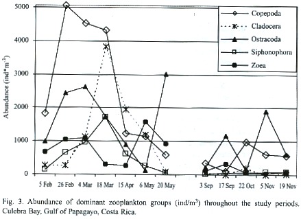
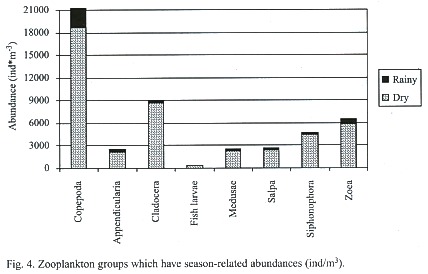
The Fig. 4 illustrates the total abundance fluctuations throughout the study periods of the dominant zooplankton groups. The higher abundance of zooplankton during the dry season is clearly visible. Like Copepoda there were peaks of abundances during the dry season 26 February – 18 March. Low abundances were recorded on 20 May, except for Ostracoda, which had high abundances at E4, E1, and E2 (Table 1). During the rainy season Copepoda and Cladocera abundances peaked on 22 October when Ostracoda abundance was at its lowest. Ostracoda abundance was highest on 17 September and 5 November.
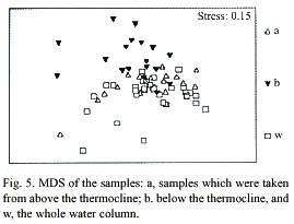
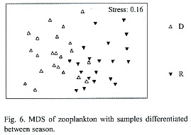
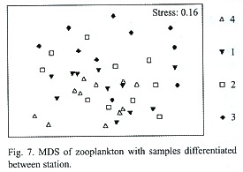
Multidimensional Scaling (MDS) graphs of zooplankton samples for the facets season and station are included in this paper. The facet for part of the water column the sample was taken from revealed the same results as for copepods alone (Fig. 5). The following MDS representations are from combined water column examination. In the case of the facet season (Fig. 6) the samples are pretty differentiated with the few exceptions being samples taken from the same station or the closest neighboring one. Analysis of the facet station (Fig. 7) did not give as clear results as the copepod species station analysis however, the same pattern of station mixing with neighboring station can still be seen and besides one outlier E4 and E3 are distinct from each other.
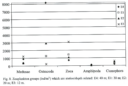
The results of the correlation matrix for zooplankton stated that season was a determining variable for the abundance of nine groups (Fig. 4). Copepoda was the order most correlated to seasonal changes with a Pearson coefficient (r) = -0.482 and p = 0.0001. zoea (r = -0.424, p = 0.0009), medusae (r = -0.419, p = 0.001), Salpa (r = -0.403, p = 0.002), Cladocera (r = -0.365, p = 0.005), Siphonophora (r = -0.345, p = 0.008), Appendicularia (r = -0.298, p = 0.023) and Branchiopoda (r = 0.456, p = 0.003) were also significantly proportional to the variable season. In these groups abundances were significantly greater in the dry season. Station depth was a determining variable for the following five groups also shown on Fig. 8: Ctenophora (r = -0.529, p = 1.93E-05), medusae (r = -0.376, p = 0.004), zoea (r = -0.350, p = 0.007), Ostracoda (r = 0.281, p = 0.033) and Amphipoda (r = 0.321, p = 0.014). At E4 (40 m) abundances of Ostracoda and Amphipoda were the highest while Ctenophora, medusae, and zoea abundances peaked at E3 (12 m). Salinity was a determining variable only for the order Ostracoda (r = 0.264, p = 0.045). Oxygen was a determining variable for three groups: Appendicularia (r = 0.379, p = 0.003), zoea (r = 0.341, p = 0.009), and barnacle naupliae (r = 0.307, p = 0.019). Two orders were influenced by temperature: Ostracoda (r = -0.391, p = 0.002) and Stomatopoda (r = 0.323, p = 0.013). The last variable, turbidity, influenced seven orders: Copepoda (r = -0.283, p = 0.031), Cladocera (r = -0.274, p = 0.037), medusae (r = -0.391, p = 0.002), Salpa (r = -0.280, p = 0.033), Siphonophora (r = -0.268, p = 0.042), zoea (r = -0.455, p = 0.0003), and Branchiopoda (r = 0.316, p = 0.016). When turbidity was high the abundance of these groups was lower as was the case if the turbidity was extremely low.
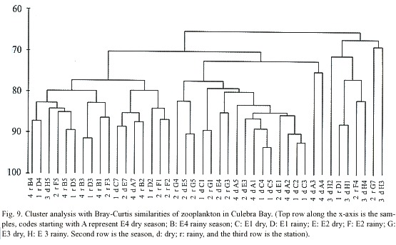
Cluster analysis (PRIMER) of zooplankton data resulted in Fig. 9. This diagram shows that samples from E4 and E1 during the dry season and samples of E1 during the rainy season are over 90% similar when analysed with the Bray Curtis coefficient of similarity. It is also interesting to note occurrences of samples which were from the same station but different seasons and over 85% similar: A7 and B2 from E4 and E5 and G5 from E2.
Discussion
Overview of hydrology: The fluctuations of zooplankton abundance and diversity in Culebra Bay are related to seasonal variations and the circulation patterns that accompany them. Upwelling occurs in Culebra Bay during the dry season (Wyrki, 1964). During this time surface waters are carried offshore by Ekman transport resulting from equatorward-blowing winds. This mixing of the shallow coastal water column causes suspension of sediments and affects the transparency of the water (Peterson, 1998). Therefore, it coincides that during upwelling, the dry season, turbididy readings were higher (lower Secchi measurements). Dominating species of upwelling systems are determined by the ability of individuals to continue their life processes while migrating in a way to remain in the upwelling system and not be carried out of their boundaries by currents (Peterson, 1998). Main characteristics of the surface water mass of an upwelling system are lowered temperatures, lowered salinity, lowered oxygen content, and high nutrient content that drives the increase in productivity (Whitledge, 1981). The temperature measurements of Culebra Bay were lower during the upwelling (dry) season. However, the average salinity was higher in the dry season, most likely because rainwater runoff from the coastal areas into the bay lowered salinity during the rainy season. Rippe (1996) also found this result in his study along the Pacific coast of Colombia.
In Culebra Bay oxygen measurements were more sporadic during the dry season due to upwelling, however the range of the measurements was nearly equal during both seasons. During some dates (i.e. May 20) in the dry season, oxygen followed the same trends as temperature in Culebra Bay – both increasing or decreasing at the same time, and having higher levels at the surface. Normally, oxygen decreases when temperature increases because less oxygen can be dissolved. The negative correlation results between temperature and salinity of Culebra Bay and those results from Rippe (1996) are evidence of this. When oxygen increases with increasing temperature, there must be higher production or increased photosynthesis by phytoplankton which could be caused by higher solar radiation and
increased nutrient levels which are optimal conditions for phytoplankton reproduction (Wetzel and Likens, 1991). High nutrient levels and turbulence characterize upwelling areas. These are also factors that promote the dominance of fast growing phytoplankton. Decreased turbulence causes phytoplankton abundance losses due to sinking. Since larger copepods utilize these larger cells more efficiently they have optimal growth rates during upwelling and an increased abundance and biomass (Landry, 1977).
Interactions with the environment: Most zooplankton normally live in well-oxygenated environments, although it has also been observed that not every copepod species is limited in diel migrations by oxyclines (Mauchline, 1998). In this study the Order Copepoda was not found to be correlated to oxygen as were Appendicularia, zoea, and Barnacle naupliae. However, two copepod species, Centropages furcatus and Acartia lilljeborgii, were found to be positively correlated with oxygen. Both species were usually limited to the water column above the thermocline.
Salinity and salinity-temperature interactions have been found to control copepod distributions and characterize geographical distributions of many species in coastal and estuarine areas. Copepods are more tolerant of changes in salinity when they are fed than when starved. Lower temperatures rather than higher ones result in higher survival rates of copepods over a broader range of salinity changes. When changes of salinity and temperature are slow, many species can acclimatize resulting in increased ranges of tolerance (Mauchline, 1998). In this study three copepod species and one Order had abundances that were correlated to salinity: Canthocalanus pauper, Centropages furcatus, Oithona plumifera and Ostracoda. On 15 April there was a decrease in salinity of 2 at E2 and E3 and the effect can be seen on all zooplankton (Fig. 2). Díaz-Zabella and Gaudy (1996) found corresponding results. They determined that most of the variations in abundance of the total zooplankton population reflected the dilution by the flushing effect of inland freshwaters in the bay.
Most calanoid copepods cannot withstand exposure to strong natural light. Strong light can also cause reduced reproductive capability and increase the mortality rates of early and late nauplier stages (Mauchline, 1998). On 5 November the lowest turbidity was recorded for all stations. The zooplankton populations at E4 and E1 peaked for the season on this date while at E2 and E3 abundance recordings were the lowest. Turbidity was higher during the dry season at E4, E1, and E2 in comparison to the rainy season. At E3 during the dry season turbidity had a higher reading on only one date – 20 May (3.2 m) in comparison to the rainy season. The average turbidity for the dry season at E3 was 4.9 m in comparison to 6.73 m during the rainy season. High turbidity during the rainy season was most likely caused by runoff from the mountains and increased outflow from the estuaries. In general, lower turbidity readings were found at the deeper stations which corresponded to the findings of Rippe (1996) who studied zooplankton the the Pacific Coast of Colombia.
The abundance of zooplankton in Culebra Bay was higher in the dry season than in the rainy season. This variation in zooplankton abundance has been seen in many studies and is often associated with physical changes in the environment (Díaz-Zaballa and Gaudy, 1996, Haridas et al. 1980, Youngbluth, 1980, and Reeve, 1970). A decrease in salinity of 2 at E2 and E3 on 15 April corresponded with a decline in the total abundance of all zooplankton. The decrease in salinity on 18 March may have caused cladocerans, which are common to neritic environments to increase in abundance (Calef and Grice, 1967). Corresponding results were found by Díaz-Zabella and Gaudy (1996) who determined during a study of La Habana Bay, Cuba that most variations in abundance of the total zooplankton population reflected the dilution by the flushing effect of inland freshwaters in the bay. Within zooplankton, Copepoda (dry season, 31%, rainy 23%) and Ostracoda (dry 19%, rainy 35%) were the main representatives of the total
abundances during both seasons - each making up roughly one-third of the total abundance of zooplankton. Huys and Boxshall (1991) stated that in terms of abundance and biomass copepods are considered the most important metazoan secondary producers in pelagic marine ecosystems. Five Orders (37% of the total zooplankton) had abundances that were correlated to stations. Abundances of Ctenophora, medusae, Ostracoda, zoea, and Amphipoda showed significant difference depending on what station the sample was from. In a similar study on the Carribean coast of Costa Rica more than 50% of all groups were associated with stations (Morales & Murillo, 1996). The same eighteen zooplankton groups were represented both off-shore (E4) and near-shore (E3) while 20 similar groups were represented at E1 and E2. During both seasons the total abundance of zooplankton and species diversity of Copepoda increased from near-shore to off-shore. Riley (1967) found that the abundance of estuarine zooplankton is higher than oceanic zooplankton but the diversity is less. Rippe (1996) found that the deeper stations had more oceanic influenced zooplankton populations. Upwelling and the modified physical conditions of the environment that accompanied it caused differences in the abundances of zooplankton to be observed in Culebra Bay.
Suggestions for future studies include a more comparative study of biomass and abundance variations, a closer examination of the other zooplankton populations, and an extended study of the effect the growing number of developments along the shore have on the zooplankton and hence, the rest of the community in the area.
Acknowledgements
This work was supported through a grant to A.M.R. (808-99-236) from the Vicerrectoría de Investigación of the Universitdad of Costa Rica and also represents a contribution to project CR-USA 808-A0-506. This work was conducted in part to fulfilment of the requeriments of a M.Sc. degree at the Center of Tropical Marine Ecology (ZMT), University of Bremen, Germany.
Resumen
La abundancia, distribución y composición del macrozooplancton fue estudiada en bahía Culebra Costa Rica (10º 38 N and 85º 40 W) en cuatro estaciones durante la época seca (Febrero-Mayo) y lluviosa (Setiembre – Noviembre) del año 2000. Las muestras fueron colectadas en intervalos de dos semanas usando una red de 500µm de poro y 0.50-m de diámetro. Copépodos (23-31%) y ostrácodos (20-34%) fueron predominantes através del año, seguidos por los cladóceros (2.5-14%), zoea (6.6-9.5%), y sifonóforos (2.5-7.2%). Altas densidades de zooplancton fueron obtenidas en Febrero y Marzo, con un pico el 18 de Marzo. Las más bajas densidades fueron observadas el 3 de Septiembre y 5 de Noviembre. Se observaron diferencias significativas en las abundancias en cada estación para los copépodos de la especie Acartia tonsa, los grupos Ctenophora, medusae, Ostracoda, zoea y Amphipoda. Comparando las estaciones seca y lluviosa, significativamente más altas densidades fueron obtenidas en todas las estaciones en la época seca; durante la época lluviosa los ostrácodos dominaron las áreas externas. La abundancia y distribución del macrozooplancton son influenciadas por el afloramiento, el cual ocurre durante la época seca en Bahía Culebra.
References
Alvariño, A. 1981. Siphonophorae. En: Boltovskoy, D. Atlas del Zooplancton Del Atlántico Sudoccidental y métodos de trabajo con el zooplancton marino. Publicación especial del INIDEP. Mar de Plata, Argentina. 936 pp. [ Links ]
Arfi, R.;G. Champalbert & G. Patrite. 1981. Systeme plantonique et pollution urbaine: an aspect des populations zooplanctoniques. Mar. Biol. 61: 133-141. [ Links ]
Bioindicators of Aquatic Ecosystem Stress. Oak Ridge National Laboratory (ORNL). 19 August 1999 <http://www.esd.ornl.gov/programs/bioindicators/ [ Links ]
Borg, I. & R. Groenen. 1997. Modern Multidimensional scaling: theory and applications. Springer-Verlag, New York, Inc. 471 pp. [ Links ]
Calef, G.W. & G.D. Grice. 1967. Influnce of the Amazon River outflow on the ecology of the western tropical Atlantic. II. Zooplankton abundance, copepod distribution, with remarks on the fauna of low salinity areas. J. Mar. Res. 25: 84-94. [ Links ]
Clarke, K.R. & R.N. Gorley. 2001. PRIMER v5: User Manual/Tutorial. PRIMER-E Ltd, UK. 90 pp. [ Links ]
Clarke, K.R. & R.M. Warwick. 1994. Change in marine communities: an approach to statistical analysis and interpretation. National Environment Research Council, UK. 144 pp. [ Links ]
Cushing, D.H. 1995. The long-term relationship between zooplankton and fish. ICES J.mar. Sci. 52:611-626. [ Links ]
Díaz-Zaballa, J. & R. Gaudy. 1996. Seasonal variations in teh zooplankton and in the population structure of Acartia tonsa in a very eutrophic area: La Habana bay (Cuba). J. Plank. res. 18:1123-1235. [ Links ]
Fujita, T.T. & S. Fujuita. 1998. Mystery of El Niño and hurricanes; overview of present, distant past and future. Wind Research Laboratory, University of Chicago. 73 pp. [ Links ]
Glynn, P., E. Druffel & R. Dunbar. 1983. A dead Central American coral reef tract: possible link with the Little Ice Age. J. Mar. Res. 41: 605.637. [ Links ]
Gross, M.G. 1993. Oceanography: A view of Earth. Prentice Hall, Englewood Cliffs. 446 pp. [ Links ]
Haridas, P., Gopala Menon, P. & M. Madhupratap. 1980. Annual variations in zooplankton from a polluted coastal environment. Mahasager-Bulletin of the National Institute of Oceanography. 13(3): 239-248. [ Links ]
Hopcroft, R.R., Roff, J.C. & D. Lombard. 1998. Production of tropical copepods in Kingston Harbour, Jamaica: the importance of small species. Mar. Biol. 130: 593-604. [ Links ]
Huys, R. & G.A. Boxshall. 1991. Copepod Evolution. Ray Soc. London, pp. 1-468. [ Links ]
Jiménez, C. 2001. Arrecifes y ambientes coralinos de Bahía Culebra, Pacífico de Costa Rica: aspectos biológicos, económicos-recreativos y de manejo. Rev. Biol. Trop. 49 (Supl. 2): 215-231. [ Links ]
Landry, M.R. 1977. A review of important concepts in the trophic organization of pelagic ecosystems. Helgoländer wiss. Meer. 30: 8-17. [ Links ]
Lindo, M.K. 1991. The effect of Kingston Harbour Outflow on the zooplankton populations of Hellshire, Southeast Coast, Jamaica. Estuarine, Coastal and Shelf Sci. 32:597-608. [ Links ]
Mauchline, J. 1998. The biology of calanoid copepods. Academic Press. San Diego. 710 pp. [ Links ]
Morales-Ramírez, A. & M. Murillo. 1996. Distribution, abundance and composition of coral reef zooplancton, Cahuita National Park, Limon, Costa Rica. Rev. Biol. Trop. 44(2): 619-630. [ Links ]
Peterson, W. 1998. Life cycle strategies of copepods in coastal upwelling zones. J. Mar. Syst. 15: 313-326. [ Links ]
Reeve, M.R. 1970. Seasonal changes in the zooplankton of south Biscayne Bay and some problems of assessing the effects on the zooplankton of natural and artificial thermal and other fluctuations. Bull. Mar. Sci. 20: 894-921. [ Links ]
Riley, G.A. 1967. The plankton of estuaries. P.: 316-326. In G.H. Lauff. (ed.). Estuaries. American Association for the Advancement of Science. Washington, D.C. [ Links ]
Rippe, L. 1996. Gemeinschaftsanalyse des Küstennahen Mesoplankton im Flachwassergebiet vor der Kolumbianischen Pazifikküste. Diplomarbeit. Universität Bremen. [ Links ]
Tester, P.A., Turner, T.T. & D. Shea. 2000. Vectorial transport of toxins from the dinoflagellate Gymnodinium breve through copepods to fish. J. Plank. Res. 22: 47-61. [ Links ]
Vandermeulen, H. 1998. The development of marine indicators for coastal zone management. Ocean & Coastal Management 39: 63-71. [ Links ]
von Wangelin, M. & M. Wolff. 1996. Comparative biomass spectra and species composition of the zooplankton communities in Golfo Dulce and Golfo de Nicoya, Pacific Coast of Costa Rica. Rev. Biol. Trop. 44 Suppl. (3): 85-105. [ Links ]
Wallace, J.M. & P. V. Hobbs, 1977. Atmospheric Science – An Introductory Survey. Academic Press, New York. 467 pp. [ Links ]
Wetzel, R.G. & G.E. Likens. 1991. Limnological analyses, 2nd ed. Springer-Verlag, Dubuque, New York. [ Links ]
Whitledge, T.E. 1981. Nitrogen recycling and biological populations in upwelling ecosystems, p.257-273. In F.A. Richards [ed.], Coastal Upwelling. Am. Geophys. Union. [ Links ]
Wyrki, K. 1964. Upwelling in the Costa Rica Dome. Fish Bull. 63: 355-372. [ Links ]
Youngbluth, M.J. 1980. Daily, seasonal, and annual fluctuations among zooplankton populations in an unpolluted tropical embayment. Estuarine and Coastal Mar. Sci. 10: 265-287. [ Links ]

