


 English (pdf)
 Article in xml format
 Article references
 Send this article by e-mail
 Cited by SciELO
  Similars in
SciELO
Similars in
SciELO  uBio
uBio 
 Permalink
Introducción
The Northern Neotropical region displays geologic and geographic complexity. It possesses one of the largest limestone platforms in the world, the karst environment extends from the lowlands of the Yucatán Peninsula to the middle- and high-altitude areas of Chiapas, Mexico (Kueny & Day, 2002; Ford & Williams, 2007; Villanueva, 2011). It is part of the largest continuous forest area left in Mesoamerica, constituting an important North-South ecological gradient (Vester et al., 2007). Due to the rapid ecosystem fragmentation and habitat loss, the area is thus interesting for study of modern and past distribution, diversity and ecology of fauna and flora (O’Brien & Pietraszek-Mattner, 1998; Pielke et al., 2007; Correa-Metrio et al., 2012; Franco-Gaviria et al., 2018). The studied lakes ecosystems from El Petén, Northern Guatemala, to the Lacandón forest and Montebello in Chiapas, Mexico span an altitudinal gradient about 100 to 1 500 m.a.s.l., with a mean annual precipitation range between 1 000 to 3 000 mm/yr across the lake sites (Moreira et al., 2007). These regions have been listed as RAMSAR sites since 2003 because, they display high biodiversity and are connected hydrologically, which highlights the importance that these lakes play in the recharge of aquifers of the sub-basin (Ramírez, 2007; Kauffer & Villanueva, 2011; Alcocer et al., 2016). In spite of the name of National Parks and RAMSAR sites, the limnological characteristics of the lakes are rare and poorly known (Alcocer et al., 2016), as well as ecological and biogeographical studies (Cohuo, Macario-Gónzalez, Pérez, & Schwalb, 2016). Although such information is needed to develop reliable paleoecological and paleoclimatic reconstructions for the region (Pérez et al., 2012, 2013; Cohuo et al., 2016; Díaz et al., 2017). Lakes of El Petén in Northern Guatemala have been previously studied probably because of their abundance, size, proximity to tourist attractions like Maya archaeological sites, and more recently, their relatively easy access (Brezonik & Fox, 1974; Deevey, Brenner, Flannery, & Yezdani, 1980; Basterrechea, 1988; Correa-Metrio et al., 2012; Pérez et al., 2013). Some paleolimnological studies have also been carried out in the region and showed that many of the lakes contain complete Holocene sediment sequences (Quexil, Salpetén, Macanché) and a few have deposits that extend well into the Pleistocene. The longest records come from deep Lake Petén Itzá (165 m) (Anselmetti et al., 2006), which appears to have held water for the last 400 ka (Kutterolf et al., 2016). A few limnological, paleoecological and palynological studied have been carried out in the Lacandón forest and Montebello region as well (Alcocer et al. 2016; Vázquez-Molina et al., 2016; Franco-Gaviria et al., 2018).
The modern study of Neotropical non-marine ostracodes ecology across an altitudinal gradient was absent until this moment. Ostracodes (Crustacea: Ostracoda) are crustaceans that are 1.5 mm long and can serve as important bioindicators in modern and paleoecological studies because: 1) they are abundant, sensitive and respond quickly to changes in environmental conditions such as temperature, conductivity and lake stage (Meisch, 2000), 2) they have calcium carbonate (calcite) valves that preserve well in lacustrine sediments, which makes them one of the best taxonomic groups for micropaleontological studies, and 3) their wide distribution and high abundance in the Northern Neotropics make them excellent paleobioindicators of past climate and environment (Canudo, 2002), 4) they also possess one of the oldest and most continuous fossil records (Griffiths & Holmes, 2000), and can thus be used to develop calibrations and infer modern and past climate and environmental conditions in the area (Pérez et al., 2012, 2013).
Therefore, our modern dataset provides ostracod-environment relationships across a broad environmental gradient, from El Petén, Guatemala to Montebello, Chiapas, Mexico. The information generated here revealed species-specific ecological preferences and provided additional environmental information on the importance of temperature and precipitation that was unknown before. Our quantitative data is applicable to reconstruction of paleoecological and paleoclimate conditions across this region, facilitating development of transfer functions to infer past temperature, conductivity and precipitation.
Materials and Methods
Study area: El Petén, Northern Guatemala, and the Lacandón forest and Montebello, in Chiapas state, Mexico are located in the Chiapas Plateau and the Gulf Coastal Plain physiographic region, which is part of the Sierra de Chiapas and Guatemala (Villanueva, 2011; Ramírez, 2007). They also correspond to the Grijalva-Usumacinta basin in Northwestern Guatemala and Southeastern Mexico and include 27 lakes. Fifteen lakes are located in El Petén, Guatemala (Yaxhá, Macanché, Oquevix, Oquevix pond, Las Pozas, Subín River, San Diego, La Gloria, Sacpuy, El Rosario, Petén Itzá, Petexbatún, Salpetén, Ixlú River, and Perdida), seven in the Lacandón forest (Yax-há, Ocotalito, Nahá, Amarillo, Lacandón, Metzabok, and T’ziBaná) and five in Montebello (Yalalush, Peñasquito, Esmeralda, Liquidambar, and Balantetic) (Table 1). The different morphometries of most of these systems were formed as a consequence of limestone (carbonate) dissolution. Although, tectonism has been involved as well, especially in highland lakes (Brenner, Rosenmeier, Hodell, & Curtis, 2002).
The studied regions are located between (15.0° - 17.1° N & 89.4° - 91.8° W), in an altitude range from 100 to 1 500 m.a.s.l. Precipitation varies across the landscape from 1 000 to 3 000 mm/yr (Fig. 1; Table 1). Most of the studied lakes were < 40 m deep, except for three lakes in El Petén: La Gloria (65 m), Macanché (80 m) and Lake Petén Itzá (165 m). Lake Balantetic in Montebello, was the highest (1 466 m.a.s.l.), and Lake Perdida in El Petén, was the lowest (75 m.a.s.l.) (Table 1). In particular, El Petén region lies at an altitude of about 110-500 m.a.s.l., with an annual average precipitation of 1 665 mm and an average annual temperature of 27 °C. Lowest monthly temperature (22 °C) in Petén is registered in January and the highest (30 °C) is in May (Pérez, 2010). The bioclimatic classification of El Petén is warm, subtropical and very humid, subtropical warm (Holdridge, 1975; Manoharan, Welch, & Lawton, 2009; Correa-Metrio et al., 2012). The mid-elevation Lacandón forest lies at an altitude of 500-950 m.a.s.l., and possesses large extensions of evergreen tropical forest, mesophilic mountain forests, coniferous forest, and secondary vegetation (Rzedowski, 2006; Vázquez-Molina et al., 2016). The climate is sub-humid and warm, with an average annual temperature of 21 °C, and an annual precipitation between 1 200 and 3 500 mm (Díaz et al., 2017). The region registers two periods of lower precipitation, between February and May, and between July and August (Kauffer & Villanueva, 2011). The Montebello lakes correspond to the highlands, lying between 1 000 and 1 500 m.a.s.l. The main plant associations are coniferous forests, broadleaf forests, mesophilic mountain forests, riparian vegetation, secondary vegetation and crop areas (Villanueva, 2011). The climate is humid temperate with rain year-round. The mean annual precipitation is 2 500 mm, and the mean annual temperature is about 17 °C. It is highly seasonal, with the coldest and warmest periods from December to February and April to September, respectively (Rzedowski, 2006; Alcocer et al., 2016; Franco-Gaviria et al., 2018).
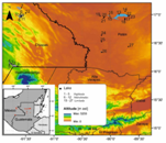
Fig. 1 Altitude and locations of studied karst aquatic ecosystems. Sampled lakes came from three altitudinal ranges: 100-500 m.a.s.l. (El Petén), 500-900 m.a.s.l. (Lacandón forest) and 1 000-1 500 m.a.s.l. (Montebello).
TABLE 1: Location, maximum depth and altitude of the study lakes, located along an altitudinal gradient from middle altitudes to the highlands from Northern Guatemala to Southern Mexico
| Region | Lake | ID | Coordinates | - | Maximum | Altitude [m | maxTempW | minTempC | Prec | PrecWet | PrecDrie |
| - | - | - | °N | °W | depth [m] | a.s.l.] | [°C] | [°C] | [mm] | [mm] | [mm] |
| Montebello | Balantetic | BAL | 16.12 | 91.78 | 3 | 1 466 | 28.7 | 10.7 | 1 961 | 191 | 125 |
| (Highlands) | Esmeralda | ESM | 16.11 | 91.72 | 5 | 1 463 | 28.7 | 10.7 | 1 961 | 191 | 125 |
| - | Peñasquito | PEÑA | 16.13 | 91.75 | 40 | 1 462 | 28.7 | 10.7 | 1 961 | 919 | 125 |
| - | Liquidambar | LIQ | 16.14 | 91.78 | 9 | 1 456 | 28.7 | 10.7 | 1 961 | 191 | 125 |
| - | Yalalush | YAL | 16.09 | 91.64 | 18 | 1 450 | 29.4 | 11.9 | 2 763 | 1 288 | 193 |
| Lacandón | Yax-há | YAXL | 16.96 | 91.59 | 32 | 930 | 30.9 | 13.8 | 2 568 | 1 154 | 202 |
| forest (Mid- | Ocotalito | OCOT | 16.95 | 91.60 | 23 | 920 | 30.9 | 13.8 | 2 568 | 1 154 | 202 |
| altitudes) | Nahá | NAH | 16.98 | 91.50 | 18 | 830 | 31.7 | 14.7 | 2 648 | 1 198 | 198 |
| - | Amarillo | AMA | 16.98 | 91.50 | 9 | 830 | 31.7 | 15.2 | 2 470 | 1 079 | 206 |
| - | Lacandón | LAC | 17.01 | 91.58 | 2 | 545 | 32.4 | 15.2 | 2 470 | 1 079 | 206 |
| - | Metzabok | MET | 17.03 | 91.50 | 20 | 543 | 33.9 | 16.6 | 2 386 | 1 052 | 194 |
| - | T'zi BaNá | TZI | 17.12 | 91.57 | 35 | 542 | 32.4 | 15.2 | 2 470 | 1 079 | 206 |
| El Petén | Yaxhá | YAX | 17.01 | 89.40 | 25 | 219 | 31.5 | 17.6 | 1 350 | 496 | 139 |
| (Lowlands) | Macanché | MAC | 16.97 | 89.64 | 80 | 165 | 31.2 | 17.5 | 1 488 | 542 | 144 |
| - | Oquevix | OQU | 15.00 | 89.74 | 10 | 148 | 33.7 | 17.8 | 922 | 474 | 15 |
| - | Pond Oquevix | TUM | 15.00 | 89.74 | 10 | 148 | 32.2 | 17.6 | 1 970 | 786 | 160 |
| - | Las Pozas | POZ | 16.34 | 90.18 | 35 | 146 | 32.4 | 17.8 | 1 817 | 735 | 143 |
| - | Subín river | SUB | 16.64 | 90.18 | 1 | 141 | 32.7 | 17.9 | 1 824 | 763 | 148 |
| - | San Diego | DIE | 16.92 | 90.42 | 8 | 134 | 32.7 | 17.9 | 1 824 | 763 | 148 |
| - | La Gloria | GLO | 16.95 | 90.37 | 64 | 132 | 32.7 | 17.9 | 1 824 | 763 | 148 |
| - | Sacpuy | SAC | 16.97 | 90.01 | 6 | 122 | 32.2 | 18.2 | 1 677 | 681 | 138 |
| - | El Rosario | ROS | 16.52 | 90.16 | 2 | 117 | 32.1 | 17.9 | 1 814 | 714 | 150 |
| - | Petén Itzá | PI | 17.01 | 89.85 | 165 | 115 | 32.3 | 18.3 | 1 511 | 596 | 129 |
| - | Petexbatún | PET | 16.44 | 90.19 | 40 | 115 | 32.2 | 17.6 | 1 970 | 786 | 160 |
| - | Salpetén | SAL | 16.97 | 89.67 | 38 | 114 | 31.8 | 18.0 | 1 523 | 578 | 138 |
| - | Ixlú river | IXL | 16.97 | 89.69 | 0.5 | 110 | 31.8 | 18.0 | 1 523 | 578 | 138 |
| - | Perdida | PER | 17.06 | 90.02 | 4 | 75 | 32.7 | 18.7 | 1 606 | 662 | 128 |
Lake name: number of samples per site. 1 Yalalush: 1; 2 Esmeralda:1; 3 Peñasquito: 1; 4 Liquidambar: 1; 5 Balantetic: 1; 6 Lacandón: 2; 7 T’zi Baná: 1; 8 Ocotalito: 2; 9 Naha: 3; 10 Amarillo: 1; 11 Yax-há: 1; 12 Metzabok: 2; 13 Petén Itzá: 16; 14 Perdida: 2; 15 Macanché: 2; 16 Yaxhá: 2; 17 Oquevix: 1; 18 Oquevix pond: 1; 19 Salpetén: 3; 20 La Gloria: 1; 21 San Diego: 2; 22 Ixlú river: 1; 23 Sacpuy: 2; 24 Subín river: 1; 25 El Rosario: 1; 26 Las Pozas: 1; 27 Petexbatún: 3.
Field work: We first collected data on ostracode habitats to generate information on their ecological preferences. We measured physical and chemical variables, the latter including cation and anion concentrations in lake waters. Samples from lakes in the Lacandón forest and Montebello sites were collected in June 2013, during the rainy season. Samples and in situ measurements from waterbodies of El Petén, Guatemala were collected during the dry season between November and February in 2005, 2006 and 2008. The data from El Petén was previously presented by Pérez (2010) and Pérez et al. (2012).
In each water body, temperature, dissolved oxygen, conductivity and pH were measured in situ using a Hydrolab Quanta (Chiapas fieldwork) or a WTW multi-parameter probe (Guatemala fieldwork) near sites where surface sediment samples were collected, i.e. in the littoral zone and deepest area. Only a single site, mostly from the littoral zone, was sampled in smaller waterbodies. In larger and deeper lakes samples were taken at different depths. Water depth was determined with a portable depth sounder. Water samples were collected with a Ruttner water sampler for chemical analysis in the laboratory. Water samples for cation analysis were fixed with nitric acid. A total of 56 surface sediment samples were collected, 35 from different depths using an Ekman grab, and 21 sediment samples were recovered from the littoral zone (0.5-1 m) using a hand net (125-µm mesh). The number of sediment samples collected from each lake is indicated in Fig. 1 and Table 2. To guarantee collection of the most recent sediments, only the top 2-3 cm from each Ekman grab were taken and preserved in 95 % ethanol.
TABLE 2: Limnological variables from the study lakes in Southern Mexico
| Region | Lake | ID | Depth | Water temperature | O2 | pH | Conductivity | Cl- | SO4 -2 | HCO3 - | Ca+2 | K+ | Mg+2 | Na+ | δ18O |
| - | - | - | [m] | [°C] | [mg/l] | - | [µS/cm] | [mg/l] | - | - | - | - | - | - | - |
| - | Yalalush | YAL2 | 18 | 20.7 | 4.1 | 7.5 | 293 | 1.7 | 1.0 | 189 | 35 | 0.2 | 18.3 | 0.4 | -5.1 |
| Highlands | Peñasquito | PEÑA2 | 40 | 18.2 | 0.1 | 7.0 | 453 | 3.0 | 40.1 | 234 | 65 | 1.0 | 17.3 | 2.1 | -6.6 |
| - | Esmeralda | ESM2 | 5 | 22.3 | 5.1 | 7.5 | 358 | 2.0 | 5.7 | 227 | 45 | 0.3 | 20.8 | 0.5 | -6.1 |
| - | Liquidambar | LIQ1 | 0.5 | nd | 8.6 | 8.3 | 485 | 7.0 | 111.7 | 134 | 73 | 3.4 | 15.0 | 6.6 | -10.0 |
| - | Balantetic | BAL1 | 0.5 | 21.9 | 6.7 | 7.5 | 712 | 12.1 | 136.7 | 285 | 116 | 4.5 | 18.2 | 14.7 | -9.5 |
| Mid-altitudes | Yax-há | YAXL1 | 0.5 | 27.3 | 6.3 | 7.5 | 235 | 2.0 | 1.3 | 134 | 31 | 0.4 | 13.5 | 0.3 | -2.3 |
| - | Ocotalito | OCOT1 | 0.5 | nd | nd | 7.8 | 275 | 1.9 | 1.6 | 173 | 27 | 0.7 | 21.4 | 0.3 | -3.2 |
| - | Ocotalito | OCOT3 | 7 | nd | nd | 7.3 | 279 | 1.9 | 3.2 | 177 | 29 | 1.0 | 20.2 | 0.4 | -2.7 |
| - | Nahá | NAH1 | 0.5 | 9.1 | 2.2 | 5.3 | 264 | 1.3 | 0.6 | 151 | 29 | 0.2 | 19.7 | 0.3 | -3.8 |
| - | Nahá | NAH4 | 5 | 24.8 | 6.4 | 7.5 | nd | nd | nd | nd | nd | nd | nd | nd | -5.6 |
| - | Nahá | NAH2 | 18 | 21.2 | 0.6 | 7.2 | 483 | 2.3 | 1.2 | 330 | 54 | 0.4 | 32.9 | 0.5 | -5.6 |
| - | Amarillo | AMA2 | 9.1 | 21.4 | 0.4 | 6.9 | 366 | 1.9 | 1.6 | 242 | 42 | 0.5 | 22.2 | 0.3 | -2.3 |
| - | Lacandón | LAC1 | 1.2 | 26.2 | 5.7 | 7.5 | 246 | 1.9 | 3.1 | 158 | 35 | 0.6 | 12.6 | 0.3 | -6.7 |
| - | Lacandón | LAC2 | 2 | 26.0 | 5.6 | 7.6 | 246 | 1.9 | 3.1 | 158 | 35 | 0.6 | 12.6 | 0.3 | -6.7 |
| - | Metzabok | MET2 | 20.1 | 26.3 | 4.1 | 7.5 | nd | nd | nd | nd | nd | nd | nd | nd | -5.1 |
| - | Metzabok | MET1 | 0.5 | 30.5 | 6.3 | 7.7 | nd | nd | nd | nd | nd | nd | nd | nd | -3.8 |
| - | T´zi BaNá | TZI2 | 35 | 20.9 | 0.1 | 7.0 | 446 | 2.3 | 7.9 | 279 | 56 | 0.5 | 26.5 | 0.5 | -5.5 |
| - | Yaxhá | YAX1 | 0.5 | 29.0 | 7.3 | 8.7 | 232 | 12.8 | 7.4 | 118 | 23 | 3.7 | 4.6 | 9.8 | 4.3 |
| Lowlands* | Yaxhá | YAX2 | 25.2 | 24.8 | 3.5 | 8.0 | 236 | 12.4 | 6.5 | 113 | 24 | 3.4 | 3.3 | 8.9 | 4.1 |
| - | Macanché | MAC1 | 0.5 | 26.8 | 5.0 | 8.1 | 850 | 41.8 | 241.8 | 287 | 44 | 5.2 | 71.3 | 21.8 | 3.3 |
| - | Macanché | MAC2 | 60 | 25.1 | 1.5 | 7.9 | 848 | 40.5 | 236.5 | 274 | 44 | 5.6 | 70.9 | 20.0 | 3.3 |
| - | Oquevix | OQU1 | 0.5 | 31.4 | 6.9 | 7.7 | 238 | nd | nd | 189 | 62 | nd | 4.2 | 4.0 | 1.3 |
| - | Pond Oquevix | TUM1 | 0.5 | 25.9 | 9.4 | 9.4 | 168 | nd | nd | 85 | 26 | nd | 1.4 | 6.5 | 5.6 |
| - | Las Pozas | POZ1 | 0.5 | 29.8 | 9.0 | 8.4 | 292 | nd | nd | 250 | 44 | nd | 30.5 | 3.4 | 1.0 |
| - | Subín river | SUB1 | 0.5 | 26.2 | 4.2 | 7.4 | 720 | nd | nd | 329 | 164 | nd | 12.1 | 9.2 | -3.3 |
| - | San Diego | DIE1 | 0.5 | 28.6 | 8.2 | 8.6 | 179 | nd | nd | 140 | 36 | nd | 2.7 | 3.8 | 1.6 |
| - | San Diego | DIE2 | 8.1 | 25.4 | 1.0 | 7.3 | 189 | nd | nd | 134 | 42 | nd | 3.4 | 4.9 | 1.3 |
| - | La Gloria | GLO1 | 0.5 | 29.2 | 8.8 | 8.6 | 186 | nd | nd | 134 | 40 | nd | 5.0 | 5.2 | 2.4 |
| - | Sacpuy | SAC1 | 0.5 | 28.8 | 8.0 | 8.4 | 285 | nd | nd | 171 | 52 | nd | 6.2 | 11.7 | 2.9 |
| - | Sacpuy | SAC2 | 5 | 26.4 | 4.4 | 7.8 | 289 | nd | nd | 207 | 52 | nd | 6.2 | 11.6 | 2.9 |
| - | El Rosario | ROS1 | 0.5 | 28.3 | 7.6 | 7.1 | 1 019 | nd | nd | 469 | 133 | nd | 47.1 | 2.9 | -4.3 |
| - | Petén Itzá | PI1 | 1 | 27.6 | 8.9 | 8.5 | 533 | 13.1 | 158.7 | 115 | 59 | 5.3 | 18.9 | 12.1 | 2.9 |
| - | Petén Itzá | PI4 | 3 | 27.4 | 8.9 | 8.5 | 532 | 13.1 | 159.8 | 115 | 66 | 6.3 | 20.6 | 13.4 | 2.6 |
| - | Petén Itzá | PI5 | 5 | 27.2 | 8.9 | 8.5 | 532 | 13.1 | 161.4 | 115 | 75 | 7.6 | 22.8 | 15.0 | 3.3 |
| - | Petén Itzá | PI6 | 10 | 27.2 | 8.9 | 8.5 | 531 | 13.0 | 149.5 | 115 | 73 | 3.9 | 20.1 | 11.4 | 3.2 |
| - | Petén Itzá | PI7 | 15 | 27.5 | 6.8 | 8.5 | 531 | 13.0 | 153.4 | 115 | 80 | 4.7 | 21.0 | 13.2 | 3.0 |
| - | Petén Itzá | PI8 | 20 | 26.8 | 6.5 | 8.5 | 529 | 13.0 | 159.9 | 116 | 82 | 6.4 | 21.1 | 12.6 | 3.7 |
| - | Petén Itzá | PI9 | 25 | 26.7 | 5.9 | 8.5 | 534 | 13.0 | 160.3 | 125 | 84 | 6.5 | 20.9 | 11.8 | 3.6 |
| - | Petén Itzá | PI10 | 30 | 26.5 | 5.3 | 8.5 | 539 | 13.0 | 160.3 | 125 | 84 | 6.5 | 20.9 | 11.8 | 3.6 |
| - | Petén Itzá | PI11 | 40 | 26.2 | 3.1 | 8.5 | 548 | 12.9 | 160.6 | 134 | 85 | 6.7 | 20.8 | 10.9 | 3.5 |
| - | Petén Itzá | PI24 | 50 | 26.0 | 3.4 | 8.4 | 547 | 12.9 | 158.7 | 128 | 81 | 6.8 | 21.0 | 12.8 | 3.7 |
| - | Petén Itzá | PI12 | 60 | 25.9 | 3.7 | 8.4 | 546 | 12.9 | 156.8 | 123 | 76 | 6.8 | 21.2 | 14.6 | 3.9 |
| - | Petén Itzá | PI13 | 80 | 25.7 | 1.7 | 8.4 | 544 | 12.9 | 157.9 | 121 | 68 | 6.7 | 21.0 | 13.0 | 3.7 |
| - | Petén Itzá | PI15 | 100 | 25.7 | 3.4 | 8.3 | 543 | 12.9 | 161.6 | 120 | 81 | 6.5 | 21.2 | 13.8 | 3.1 |
| - | Petén Itzá | PI16 | 120 | 25.6 | 2.0 | 8.3 | 544 | 12.9 | 158.9 | 118 | 85 | 6.1 | 26.1 | 10.8 | 3.0 |
| - | Petén Itzá | PI17 | 140 | 26.1 | 2.0 | 8.2 | 541 | 12.9 | 157.3 | 125 | 75 | 4.0 | 19.5 | 6.8 | 3.1 |
| - | Petén Itzá | PI2 | 160 | 25.8 | 1.5 | 8.1 | 544 | 12.9 | 157.4 | 121 | 65 | 3.7 | 19.3 | 7.9 | 3.0 |
| - | Petexbatún | PET1 | 0.5 | 30.9 | 9.7 | 8.0 | 568 | nd | nd | 293 | 74 | 0.0 | 40.2 | 4.9 | -2.9 |
| - | Petexbatún | PET5 | 5 | 30.9 | 9.7 | 8.0 | 568 | nd | nd | 354 | 166 | 0.0 | 48.1 | 5.6 | -3.5 |
| - | Petexbatún | PET2 | 40 | 30.9 | 6.0 | 11.3 | 1 225 | nd | nd | 409 | 179 | 0.0 | 47.1 | 6.8 | -3.8 |
| - | Salpetén | SAL1 | 0.5 | 29.7 | 8.4 | 8.2 | 4 310 | nd | nd | 122 | 801 | 0.0 | 351.1 | 142.1 | 4.6 |
| - | Salpetén | SAL4 | 15 | 25.6 | 1.6 | 7.5 | 4 290 | nd | nd | 171 | 893 | 0.0 | 410.0 | 156.8 | 4.6 |
| - | Salpetén | SAL2 | 37.5 | 25.4 | 0.8 | 7.3 | 4 250 | nd | nd | 140 | 796 | 0.0 | 360.7 | 148.2 | 4.7 |
| - | Ixlú river | IXL1 | 0.5 | 25.9 | 6.7 | 7.5 | 1 025 | nd | nd | 433 | 238 | 0.0 | 59.8 | 64.4 | -3.9 |
| - | Perdida | PER1 | 0.5 | 28.8 | 9.8 | 8.8 | 232 | 4.2 | 15.1 | 131 | 43 | 3.8 | 2.2 | 2.7 | 0.4 |
| - | Perdida | PER2 | 4.3 | 26.0 | 7.8 | 8.6 | 234 | 4.2 | 14.9 | 123 | 35 | 1.9 | 2.1 | 4.8 | 0.6 |
Information modified from Pérez et al. (2010, 2012). ID numbers are random and do not indicate the number of samples taken per lake. No data (nd)
Laboratory work (Ostracode analysis): Modern sediment samples were taken to determine ostracode species composition and relative abundances (Appendix 1). From each of the 56 sediment samples, 5 cm3 were subsampled, sieved using a 63-µm mesh size, and all adult and juvenile ostracode carapaces and valves (broken and intact) were picked using fine brushes and stored on micropaleontological slides. Valves were photographed and measured using scanning electron microscopy (SEM), Hitachi SU 1510 at Laboratorio de Microscopía y Fotografía de Biodiversidad, Instituto de Biología, Universidad Nacional Autónoma de México (Appendix 2, Appendix 3). Carapaces with well-preserved soft parts were stored in Eppendorf vials with 95 % ethanol and then dissected and mounted following methods described by Danielpol et al. (2002). Ostracode species were identified using Pérez et al. (2010, 2012) and Cohuo et al. (2016) descriptions and literature elsewhere. Here we used the most current species names suggested by Cohuo et al. (2016): Cypria petenensis (Ferguson et al., 1964) [previously referred as Physocypria globula (Furtos, 1933)], Cypridopsis vidua (O.F. Müller, 1776) [previously referred as C. okeechobei (Furtos, 1936)], Heterocypris putei (Furtos, 1936) [previously referred as H. punctate (Keyser, 1975)], and Paracythereis opesta (Brehm, 1939) [previously referred as Limnocythere opesta (Brehm, 1939)].
Water chemistry: Concentrations of major cations (Ca2+, Mg2+, Na+, K+) and anions (HCO3 -, SO4 -2, Cl-) were determined in all collected water samples, following standard procedures (APHA, 1995, 1998, 2005; Armienta et al., 2008). Analyses were conducted at Laboratorio de Química Analítica, Instituto de Geofísica, Universidad Nacional Autónoma de México. Oxygen isotope values were measured on water samples from the Lacandón and Montebello lakes using a Picarro L2120-I Isotopic Liquid Water and Water Vapor Analyzer coupled with a Picarro A0211 High Precision Vaporizer and a CTC HTS PAL auto-sampler. Measurements were done at the University of Florida (UF) and results were standardized based on two internal UF water standards (Beta and Gamma) that were calibrated using international standards (V-SMOW, V-SLAP, and V-GISP). Oxygen isotope values on water samples from El Petén lakes were measured at UF using a VG/Micromass (now GV Instruments) PRISM Series II isotope ratio mass spectrometer (Pérez, 2010). All isotope results are reported in standard delta notation relative to Vienna Standard Mean Ocean Water (VSMOW).
Environmental data was standardized using standard deviations. Diversity values were calculated using the Shannon index for each study site, displaying the heterogeneity of communities using: 1) the number of species present (S = richness), and 2) their relative abundances (equitability) (Krebs, 1989; Moreno, 2010). The biological diversity is expressed as eH/S, where the greater the difference between eH and S, the less diverse the community is (Jost, 2006).
The most significant variables for the subsequent Canonical Correspondence Analysis (CCA, Fig. 2) were selected using a Principal Component Analysis (PCA, Fig. 3A). PCA included 13 limnological variables (water lake temperature, dissolved oxygen, pH, conductivity, water depth, 18O, Ca+2, K+, Mg+2, Na+, SO4 -2, Cl-, HCO3 -) and five regional environmental variables (maximum air temperature of the warmest month, minimum air temperature of the coldest month, annual precipitation, precipitation of the wettest quarter, precipitation of the driest quarter) extracted from the climate data base WorldClim (Fick & Hijmans, 2017) which is often used in species distribution modeling and related ecological modeling techniques. The environmental data were standardized using standard deviations. The PCA suggested a correlation between conductivity and Ca+2, Na+, Mg+2; between lake temperature and minimum air temperature of the coldest month, δ18O; between annual precipitation and precipitation of the wettest quarter, precipitation of the driest quarter; and between K+ and ions Cl-, SO4 -2. According to the PCA, conductivity, minimum air temperature of the coldest month, maximum air temperature of the warmest month, annual precipitation, HCO3 -, pH, and related ions Cl-, SO4 -2 and K+ were the most variable environmental attributes of the study region and were therefore selected them for further analyses to avoid undesirable effects of highly correlated variables.
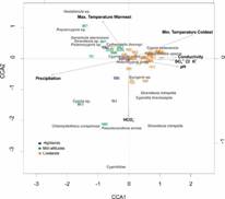
Fig. 2 Canonical Correspondence Analysis (CCA). The figure shows site ordination based on the ostracode species (in italics) and environmental variables (maximum and minimum air temperature of the warmest and coldest month, conductivity, water chemistry (K+, SO4 -2, Cl-), pH, HCO3 -, and annual precipitation. Arrows represent the most significant environmental variables identified previously by the PCA (Fig. 3A).
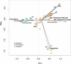
Fig. 3A Principal Component Analysis (PCA) using limnological and regional environmental variables. The figure shows site ordination based on 13 limnological variables (water lake temperature, dissolved oxygen, pH, conductivity, water depth, δ18O, Ca+2, K+, Mg+2, Na+, SO4 -2, Cl-, HCO3 -) and 5 regional environmental variables (maximum air temperature of the warmest month, minimum air temperature of the coldest month, annual precipitation, precipitation of the wettest quarter, precipitation of the driest quarter) extracted from the climate data base WorldClim. Arrows and names in black represent the most significant environmental variables identified for further analysis. For species IDs and full names see Table 3.
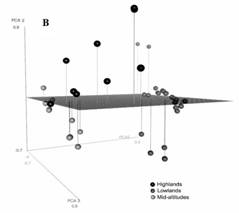
Fig. 4B Principal Component Analysis sample scores for studied lakes. Sites are color coded by regional provenance (black: Montebello [coldest], dark gray: El Petén [warmest], and light gray: Lacandón forest [intermediate temperature]).
TABLE 3: Ostracode species frequencies (occurrence) and richness (S) in the study lakes
| Ostracode species | - | EUC | CUN | CBR | VES | CPD | POT | CYA | SMA | STR | SIN | KEY | CPE | HPU | POP | DST | PAN | CIL | CVI | S |
| - | Yalalush | - | - | - | - | x | - | - | - | - | - | x | - | - | - | x | x | - | x | 5 |
| Highlands | Peñasquito | - | - | - | - | - | - | - | - | - | - | x | - | - | - | x | x | x | x | 5 |
| - | Esmeralda | - | - | - | - | x | - | - | - | - | - | - | - | - | - | x | x | x | x | 5 |
| - | Balantetic | - | - | - | - | - | - | - | - | - | - | x | - | - | - | x | x | - | x | 4 |
| - | Liquidambar | - | - | - | - | - | - | - | - | - | - | - | - | - | - | - | - | - | x | 1 |
| - | Nahá | - | x | - | x | - | x | x | - | x | - | x | - | x | - | x | x | x | x | 11 |
| - | Metzabok | - | - | - | x | - | - | x | - | x | - | x | - | - | - | x | x | x | x | 8 |
| Mid- | Ocotalito | - | - | - | - | - | x | - | - | - | - | - | - | - | - | x | x | x | - | 4 |
| altitudes | T´zi BaNá | - | - | - | - | - | - | x | - | - | - | x | - | - | - | - | - | x | x | 4 |
| - | Yax-há | - | - | - | - | - | - | - | - | - | - | - | - | - | - | - | - | x | - | 1 |
| - | Amarillo | - | - | - | - | - | - | - | - | - | - | - | - | - | - | - | - | - | - | 0 |
| - | Lacandón | - | - | - | - | - | - | - | - | - | - | - | - | - | - | - | - | - | - | 0 |
| - | Macanché | - | - | x | - | - | - | - | - | - | x | - | x | - | x | x | x | x | x | 8 |
| Lowlands* | El Rosario | x | - | - | - | - | x | - | - | - | - | - | x | x | - | x | X | x | x | 8 |
| - | Petén Itzá | - | - | - | - | - | - | - | - | - | x | - | x | x | x | x | X | x | x | 8 |
| - | Petexbatún | - | - | - | - | - | - | - | - | - | x | - | x | x | x | x | X | x | x | 8 |
| - | Salpetén | - | - | - | - | - | - | - | - | - | x | - | x | x | x | - | X | x | x | 7 |
| - | Sacpuy | - | - | - | - | - | - | - | - | - | - | - | x | x | x | x | - | x | x | 6 |
| - | Perdida | - | - | - | - | - | - | - | - | - | - | - | - | x | x | x | - | x | x | 6 |
| - | Yaxhá | - | - | - | - | - | - | - | - | - | - | - | x | - | x | - | X | x | x | 5 |
| - | Oquevix pond | - | - | x | - | - | - | - | x | x | - | - | - | x | - | - | - | - | - | 4 |
| - | Subín river | - | x | - | - | - | - | - | x | - | - | - | - | - | - | - | - | x | x | 4 |
| - | Las pozas | - | - | - | - | - | - | - | - | - | - | - | - | - | x | - | x | - | x | 3 |
| - | Ixlú river | - | - | - | - | - | - | - | x | - | - | - | - | - | - | x | - | - | x | 3 |
| - | Oquevix | - | - | - | - | - | - | - | - | - | - | - | - | - | - | - | - | - | x | 1 |
| - | La Gloria | - | - | - | - | - | - | - | - | - | - | - | - | - | - | - | - | - | x | 1 |
| - | San Diego | - | - | - | - | - | - | - | - | - | - | - | - | - | - | - | - | - | - | 0 |
| Species frequency | - | 1 | 2 | 2 | 2 | 2 | 3 | 3 | 3 | 3 | 4 | 6 | 7 | 8 | 8 | 14 | 15 | 16 | 21 | - |
Species are ordered from lower to higher frequencies (left to right). A species frequency (bottom row) equal to 1 means that species is restricted to a single lake, whereas high frequency values indicate that the species is widely distributed. Species richness (right column) indicates the number of species in each lake. Benthic species are highlighted in gray, whereas the rest are nektobenthic tax. Information from Pérez et al. (2010, 2011). Chlamydotheca unispinosa (CUN), Cypretta brevisaepta (CBR), Cypria petenensis (CPE), Cypria sp. (CYA), Cyprididae* (CPD), Cypridopsis vidua (CVI), Cytheridella ilosvayi (CIL), Darwinula stevensoni (DST), Eucypris sp. (EUC), Heterocypris putei (HPU), Keysercypria sp. (KEY), Paracythereis opesta (POP), Potamocypris sp. (POT), Pseudocandona antillana (PAN), Stenocypris major (SMA), Strandesia intrepida (SIN), Strandesia sp. (STR), Vestalenula sp. (VES).
A CCA (Fig. 2) (Legendre & Legendre, 2003) was performed to determine the environmental variable(s) that best explain ostracode distribution across the karst altitudinal gradient. Analysis used 51 sediment samples, 24 study waterbodies, and all species (n = 18). We did not include the sediment samples from Lakes Amarillo (n = 1), Lacandón (n = 2) (mid-altitude), and San Diego (n = 2) (lowlands), where ostracodes were absent. The most significant environmental variables identified by the PCA (maximum air temperature of warmest month, minimum air temperature of the coldest month, conductivity, pH, precipitation, HCO3 - and other ions [K+, SO4 -2, Cl-]) were also included. We also considered the spatial effect (i.e. latitude, longitude and altitude) in the analysis. It, however, was a co-variable of other environmental variables presented here, so is not shown in the graphs. The behavior of the species across environmental gradients was described using locally weighted scatterplot smoothing (non-parametric LOESS regression) (Correa-Metrio, Bush, Pérez, Schwalb, & Carera, 2011). Only species distributed along the whole altitude range were considered Darwinula stevensoni (Brady & Robertson, 1870), Pseudocandona antillana (Broodbakker, 1983), Cytheridella ilosvayi (Daday, 1905) and, Cypridopsis vidua (O.F. Müller, 1776). All the analyses were performed using the Project R software (R Core Team, 2013) and CorelDraw X7 (Golden Software Inc., 2012).
Results
Karst aquatic ecosystems across an altitude gradient in Mexico and Guatemala: Table 1 and Table 2 displays values for all limnological and regional environmental variables determined for each lake and sampling site. Surface water temperatures ranged from 21.2 °C (Yalalush) to 30.5 °C (Metzabok) and 31.4 °C (Oquevix), and dissolved oxygen from 4.1 (Metzabok and Yalalush) to 8.6 mg/l (Liquidambar). The highest value was 9.8 mg/l in Lake Perdida. Generally, shallow lakes displayed warmest waters. Stable oxygen isotope values (δ18O) in waters ranged from -10.06 ‰ (Liquidambar) to -2.69 ‰ (Ocotalito), to 5.6 (Oquevix pond). Studied lakes had neutral pH values, near 7 (Amarillo, Peñasquito and El Rosario), to alkaline values of about 9.4 (Oquevix pond). Conductivity values of the lake waters displayed a range from 168 µS/cm (Oquevix pond) to 4 310 µS/cm (Salpetén). Elsewhere, 246 µS/cm (Lacandón) and 712 µS/cm (Balantetic) were the minimum and maximum conductivity values for mid-altitude and highland lakes, respectively. Sulfate was highest in Lake Balantetic (137 mg/l) and Lake Macanché (242 mg/l), magnesium concentration was highest in Nahá (30 mg/l), and bicarbonate was highest also in Balantetic (285 mg/l). Lake Balantetic also displayed the highest concentration of chloride (12.1 mg/l), potassium (4.5 mg/l), and sodium (14.7 mg/l), which explains its overall high conductivity. In the lowlands of El Petén, highest individual ion concentrations were as follow: magnesium (351 mg/l) in Lake Salpetén, bicarbonate (470 mg/l) in Lake El Rosario, chloride (42 mg/l) in Lake Macanché, potassium (7.6 mg/l) in Lake Petén Itzá, and sodium (142 mg/l) in Lake Salpetén. In general, the highland lakes of Montebello were characterized by higher sulfate concentrations, compared to the mid-elevation lakes. Lowland lakes from El Petén, Northern Guatemala, also display higher sulfate concentrations and generally higher conductivities than lakes at higher elevations.
Species richness, diversity and distribution across environmental gradients in karst Southern Mexico and Guatemala: A total of 18 ostracode species were identified in this study (Table 3; Appendix 2, Appendix 3). Most species are nektobenthic and only five are benthic. Undetermined specimens from the family Cyprididae (Baird, 1845) were restricted to the highland of Montebello. Because only valves (juveniles A-8, A-7) were found, we did not attempt to infer its ecological preferences. Table 4 displays ostracode species frequency and richness (S) for each lake. Lakes with the highest species richness were Yalalush, Peñasquito, and Esmeralda (S = 5, highlands), Nahá (S = 11, mid-altitude), and Macanché, El Rosario, Petén Itzá, and Petexbatún (S = 8, lowlands). Generally, higher S values were reported from mid-elevation. Ostracodes were absent in Lakes Amarillo and Lacandón (mid-altitude), and San Diego (lowlands). One ostracode species was found in only a single lake: Eucypris sp. (El Rosario, lowlands lake). Four widely distributed species were: Darwinula stevensoni (Brady & Robertson, 1870), Pseudocandona antillana (Broodbakker, 1983), Cytheridella ilosvayi (Daday, 1905), and Cypridopsis vidua (O.F. Müller, 1776). Frequently encountered species included Cypria petenensis (Ferguson et al., 1964) (7 lakes), Heterocypris putei (Furtos, 1936) (8 lakes), Paracythereis opesta (Brehm, 1939) (8 lakes), D. stevensoni (14 lakes), P. antillana (15 lakes), C. ilosvayi (16 lakes), and C. vidua (21 lakes). Cypria petenensis, H. putei and P. opesta are characteristic species from the lowlands of El Petén (Pérez, 2010) and the mid-elevation lake of Nahá, Lacandón forest, however abundances are substantially higher in the lowlands. Cypria sp., and Vestalenula sp. are restricted to the mid-altitude lakes of the Lacandón forest. Finally, unidentified specimens from the family Cyprididae (Baird, 1845) were found in the upland lakes of Montebello. Greatest species diversity (H) was found in the Lacandón forest. Lake Nahá (H = 1.9), followed in diversity (H = 1.5) by highland lake Esmeralda, and lowland lakes Sacpuy, El Rosario, Petén Itzá, and Petexbatún (Table 4). In general, lakes from Lacandón forest were lightly more diverse (Haverage = 1.09) than those of the lowland El Petén and the Montebello highlands (Haverage = 0.94).
TABLE 4: Ostracode abundance (valves 5 cm3 wet sediment) and diversity index (H) for each study lake
| - | Highlands | - | - | - | - | Mid-altitudes | - | - | - | - | - | - | Lowlands | - | - | - | - | - | - | - | - | - | - | - |
|---|---|---|---|---|---|---|---|---|---|---|---|---|---|---|---|---|---|---|---|---|---|---|---|---|
| - | YAL | PEÑA | ESM | LIQ | BAL | YAXL | OCOT | NAH | MET | XIB | YAX | MAC | OQU | TUM | POZ | SUB | GLO | SAC | ROS | PI | PET | SAL | IXL | PER |
| Taxa_S | 5 | 5 | 5 | 1 | 4 | 1 | 4 | 11 | 8 | 4 | 5 | 8 | 1 | 3 | 3 | 4 | 1 | 6 | 8 | 8 | 8 | 7 | 3 | 6 |
| Individuals | 47 | 43 | 42 | 1 | 43 | 4 | 24 | 2 633 | 1 171 | 352 | 115 | 395 | 7 | 4.09 | 3 | 2 | 17 | 64 | 444 | 3 806 | 59 | 1 961 | 6.18 | 51 |
| Dominance_D | 0.3 | 0.4 | 0.3 | 1.0 | 0.7 | 1.0 | 0.4 | 0.2 | 0.3 | 0.4 | 0.8 | 0.4 | 1.0 | 0.5 | 0.3 | 0.5 | 1.0 | 0.3 | 0.3 | 0.3 | 0.3 | 0.6 | 0.5 | 0.4 |
| Shannon_H | 1.4 | 1.3 | 1.5 | 0.0 | 0.6 | 0.0 | 1.1 | 1.9 | 1.5 | 1.1 | 0.5 | 1.2 | 0.0 | 0.8 | 1.1 | 0.8 | 0.0 | 1.5 | 1.5 | 1.5 | 1.5 | 0.9 | 0.7 | 1.3 |
| Biological diversity (eH/S) | 0.8 | 0.7 | 0.9 | 1.0 | 0.5 | 1.0 | 0.7 | 0.6 | 0.5 | 0.7 | 0.3 | 0.4 | 1.0 | 0.7 | 1.0 | 0.5 | 1.0 | 0.7 | 0.5 | 0.5 | 0.5 | 0.3 | 0.7 | 0.6 |
| H average | 0.94 | - | - | - | - | 1.09 | - | - | - | - | 0.94 | - | - | - | - | - | - | - | - | - | - | - | - | - |
The greater the difference between eH and S, the less diverse the community
Relationship between ostracode abundance and environmental variables: The PCA was used to identify correlations between environmental variables (Fig. 3A). The first and second components explained 54 % of the total data variance. The first component (33 % of the original variance) was apparently associated with temperature and precipitation. The second component (21 % of the original variance) was apparently associated with conductivity and related ions. This analysis revealed that annual precipitation, water chemistry (SO4 -2, Cl-, and K+), maximum and minimum air temperature of the warmest and coldest month, respectively, and conductivity, represent the widest environmental gradients along El Petén, the Lacandón forest and Montebello. Studied lakes were ordered across a well-defined temperature gradient (Fig. 3B), with the warmest sites (highest scores on Axis 1) corresponding to El Petén, Northern Guatemala. Sites with intermediate temperatures included those from the Lacandón forest, and Montebello displayed the coldest temperatures, with the lowest scores on Axis 1.
The CCA (Fig. 2) showed that minimum air temperature of the coldest month, conductivity, related ions (Cl-, SO4 -2 and K+), pH, and precipitation are the variables that best explain ostracode distributions in the study area (Axis 1), followed by maximum air temperature of the warmest month, and HCO3 - (Axis 2). The Lacandón forest and Montebello lakes were mostly located in the upper left positive quadrant and the warmer sites (lowlands) appear in the right quadrants. Most lowland sites displayed higher conductivities and minimum air temperatures of 17 to 18 °C. The total explained variability was 48 % and the explained variance of Axis 1 and 2 was of 42 % (species) and 92 % (environmental variables). This analysis also revealed that there are ostracodes indicative of warmer temperatures (C. petenensis, P. opesta, Cypridopsis vidua, Eucypris sp., Strandesia intrepida (Furtos, 1936), and Cypretta brevisaepta (Furtos, 1934)). Species associated with mid-temperatures (Lacandón forest) are Cypria sp., Chlamydotheca unispinosa (Baird, 1862), Pseudocandona antillana (Broodbakker, 1983), Vestalenula sp., Keysercypria sp., Darwinula stevensoni (Brady & Robertson, 1870), Strandesia sp., and Potamocypris sp.
LOESS regressions were used to explore the response of species to the most significant environmental variables (Fig. 4), which included maximum air temperature of the warmest month, minimum air temperature of the coldest month, conductivity, HCO3 -, annual precipitation, and pH, the four most frequent (number of lakes with the species) and widely distributed (geographically widespread) ostracode taxa were considered for these regressions (D. stevensoni, C. viuda, Cytheridella ilosvayi and P. antillana). Analysis revealed that temperature preference was similar among two species. C. ilosvayi, and P. antillana displayed higher abundances in temperatures ranges, from 31 to 33 °C, and tolerated coldest temperature from 12 to 18 °C, whereas, C. vidua is more abundant in warmer temperatures. Results for conductivity show that P. antillana was found in sites with lower conductivity values (< 1 000 S/cm) and C. ilosvayi displays higher abundance when conductivities exceed 2 000 S/cm. Cypridopsis vidua abundances increase with conductivity, whereas D. stevensoni inhabits a wider conductivity range and also tolerated wider HCO3 - values (100 to 400 mg/l), as did C. ilosvayi. P. antillana was more abundant at 300 mg/l. Darwinula stevensoni and P. antillana were more abundant at mid-altitudes with precipitation values between 2 000 and 2 500 mm/yr. Moreover, the analysis showed that C. ilosvayi and C. vidua are the most tolerant species and are found in lakes where precipitation ranges from 1 000 to 2 500 mm/yr. With reference to the pH, D. stevensoni displays higher abundance at pH 7-8, whereas P. antillana is indicative of pH = 7. Cytheridella ilosvayi and C. vidua are present in a wider pH range, from 7 to 9.
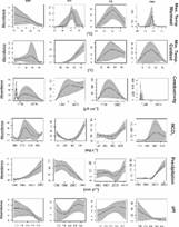
Fig. 5 LOESS regressions. Based on the PCA analysis (Fig. 3A) ostracode response to the maximum air temperature of the warmest month, minimum air temperature of the coldest month, conductivity, HCO3 -, precipitation, and pH. The mean of the species response is shown as a solid black line. The gray area shows the dispersal species response between 0.025 and 0.975 validation (black dashed lines). For species IDs and full names see Table 3. The species represented here are those found along the entire altitudinal gradient (Table 4).
Discussion
Karst aquatic ecosystems from El Petén, Guatemala, the Lacandón forest and Montebello, Mexico: Even though all our study lakes lie in karst terrain, they displayed large differences in morphology, maximum depth and surface temperature, determining many of its limnological characteristics (Table 1). As expected in this karst environment, all lake waters displayed high concentrations of bicarbonate, calcium, magnesium, and sulfate, and neutral to alkaline pH (Cohuo et al., 2016). The increase of bicarbonate is associated with a decrease of the allochthonous silicate fraction (Battistel et al., 2018). It is reasonable that the higher rainfall during the wet season favor the transport of silicate material into the lake, while higher lake levels dilute carbonates and prevent their precipitation. The higher ionic strength observed in the lowlands could be explained by higher evaporation rates and surface temperatures (Pérez et al., 2013), but may also reflect localized deposits of evaporite minerals in some El Petén watersheds. Temperatures and stable isotope values in lake surface waters are probably explained by the altitude gradient. It is well known that lower δ18O values suggest higher lake levels (Rosenmeier et al., 2002), explain by a negative balance between evaporation (E) and precipitation (P) (Curtis, Brenner, & Hodell, 1998). Disparities in E/P at different altitudes explain the limnological differences between lakes of the El Petén lowlands, the mid-elevation Lacandón forest and the Montebello highlands. This is illustrated by comparing the stable isotope values of lake waters from these three areas, with more negative values at higher elevations (Table 2). The highest values shown by Lake Balantetic, Montebello, with respect to conductivity, chloride, calcium, potassium, and sodium, can be explain because this lake has been classified as an uvala (Alcocer et al., 2016). Uvalas typically display elliptical, i.e. elongate shapes, as they are formed by two or more coalesced dolines. Lake Balantetic lowest mean width (0.23 km), depth (< 3 m), and small superficial area (13.6 ha) (Alcocer et al., 2016) has an important effect on determinate the chemical parameters, as well as the movement of water within the lake, and the sedimentary inputs from the drainage basin (Wetzel, 2001).
Ostracodes diversity across an altitudinal gradient: The ostracode fauna of the study area reflects the limnological heterogeneity of the region, displaying different distributional patterns and ecological preferences. Cypridopsis vidua (O.F. Müller, 1776), Cytheridella ilosvayi (Daday, 1905), Pseudocandona antillana (Broodbakker, 1983), and the cosmopolitan species Darwinula stevensoni (Brady & Robertson, 1870; Cohuo et al., 2016; D’ Ambrosio, García, Díaz, Chivas, & Claps, 2017) are the most tolerant species and are distributed across the entire altitudinal gradient (Table 4). They show great morphological variability, which may allow them to adapt to a wide range of environmental conditions (Gandolfi, Benedetta, Van Doninck, Rossi, & Menozzi, 2009; Cohuo et al., 2016). The identification of tolerance species, are important for paleoecological investigations, because they can serve as modern analogues for reconstructing the Quaternary history of the area. The great abundance of Cypria petenensis (Ferguson et al., 1964), Heterocypris putei (Furtos, 1936) and Paracythereis opesta (Brehm, 1939) in the lowlands can be associated to habitats with higher surface water temperatures, primarily in littoral zones with abundant macrophytes (Pérez et al., 2012). Thus, seems to be a good indicators of low lake levels (< 40 m). Although there is evidence that C. petenensis is a species able to tolerate deeper waters (< 60 m). Specifically, H. putei is known to be distributed in Yucatán Peninsula, Mexico, Northern Guatemala, and Belize (Cohuo et al., 2016). Moreover, P. opesta has been reported as a thermocline indicator (Pérez et al., 2012). Finally, C. petenensis as well as P. opesta have been reported in Central Southern Yucatán Peninsula and Belize (Cohuo et al., 2016). Our data demonstrate that the mid-elevation lakes are more diverse (Table 4), suggesting that this region has a high potential for harboring microrefugia. This is due the intersection of two biogeographic zones across steep environmental gradients, where Neotropical taxa from Central America and the Yucatan Peninsula intermingle with Nearctic elements from Central Mexico (Bush, 2002; Correa-Metrio, Meave, Lozano-García, & Bush, 2014; Franco-Gaviria et al., 2018). In contrast, the low diversity found in Montebello highlands, may be explained by the higher altitude, lower temperature, and higher erosion, as well as variables we did not consider, such as abundance of aquatic macrophytes, contamination, predation by fish and invertebrates, among other factors (Pérez, 2010; Olea-Olea & Escolero, 2015). The most plausible explanations for the lack of ostracodes in Lakes Amarillo and Lacandón (mid-altitude), and San Diego (lowlands) is 1) a structural difference of habitats, where there are zones with a more homogeneous habitat and less resources of food (Hernández, Escobar, & Alcocer, 2010); 2) a high abundance of Cladocera, a taxon that has been observed as competitor for ostracodes (Umaña-Villalobos, Avilés-Vargas, & Esquivel-Garrote, 2018).
Ostracodes ecology - temperature, conductivity, and precipitation indicators: These gradients are most likely associated with the steep altitudinal gradient of the region (Fig. 3A, Fig. 3B). Thus, it was expected that the ostracodes fauna would respond to these variables, an observation confirmed by the CCA (Fig. 2). The distribution of samples along the first three axes of the PCA (Fig. 3B) suggests that air temperature plays an important role in structuring the regional environmental gradients. Previous studies focused on the lowlands reported that conductivity and water depth were the main controlling variables in that environment (Pérez, 2010; Pérez et al., 2013). Our examination across this altitude gradient revealed that additional variables are important influences on tropical ostracodes. Precipitation and altitude are directly related in the study area (Fig. 1) (Pérez et al., 2010) and data analyses showed that precipitation is one of the most important variables controlling ostracodes, influencing inversely pH and conductivity. The hydrologic balance in areas across Mexico is described by the relative amount of evaporation (E) to precipitation (P). The Mexican deserts, the inner Northern basin and most of the Yucatán Peninsula lowlands display a negative moisture balance, that is E > P (Pérez, 2010). The different moisture balances across this latitudinal gradient explain the differences observed in the lakes and therefore the presence/absence of ostracodes species. It might be assumed that temperature would not be an important variable in the tropics because differences between lowland and highland sites are relatively small. For instance, Pérez et al. (2011) reported in the lowlands surface water temperatures from 21.6 to 32.0 °C (range = 10.4 °C), which is small relative to water temperature ranges compared with higher latitudes. Nevertheless, ostracodes development depends on water temperature (Mezquita, Roca, & Wansard, 1999; Smith & Delorme, 2010), our results suggest that maximum and minimum air temperature of the warmest and coldest month are a factor that influences ostracodes distribution and abundance in the study area. The inclusion of the air temperature allows to cover all the temporality in which the species develop. For example, the distribution of species from the Northern hemisphere may be limited in its Southern extension by the highest average temperatures in July (summer) that adults can tolerate, but its extension to the north could be more influenced by minimum winter temperatures (January) in which eggs at rest can survive (Horne, 2008). This approach can be a solution to avoid seasonal sampling, where access to the research areas are difficult and resources are limited. It has been demonstrated that species occurrences can be defined usefully in terms of the geographical distribution of mean July and January air temperature ranges. Therefore, using the WorldClim data set to calibrate species’ temperature ranges might facilitate an estimation of past air temperatures (Horne, 2007), allowing thus more detailed paleoclimate reconstructions.
LOESS regressions yielded species ecological information for the benthic Darwinula stevensoni, Cytheridella ilosvayi, Pseudocandona antillana and nektobenthic Cypridopsis viuda. Due to D. stevensoni has a cosmopolitan distribution, this has been shown to be a highly tolerant specie (Cohuo et al., 2016). Regardless of their life stage or type of habitat, showed high survival values even in extreme conditions (D’ Ambrosio et al., 2017). Different studies indicated higher abundances in sites with precipitation from 2 000 to 2 500 mm/yr, a broad range of conductivities, and temperatures less than 32 °C (Gandolfi et al., 2009). Our results suggest an association more to cooler temperatures (28 ºC) and lower conductivities (1 500 mm/yr), which contributes to reinforce its high tolerance range estimated globally. Cytheridella ilosvayi displays a wider precipitation and conductivity range (1 000-2 500 mm/yr and 1 000-3 000 µS/cm, respectively). This specie also tolerates high temperatures values (32 °C). Our results allow us to confirm previous observations that show that this specie is an indicator of warm and humid conditions (Pérez et al., 2012). As for P. antillana shows a preference for sites with higher precipitation (2 000-2 500 mm/yr), lower conductivity (< 1 000 µS/cm) and lower temperatures (14 °C). Therefore, it is possible to consider this specie as an indicator of cold and humid conditions. Finally, C. vidua, regression analysis suggests that is most abundant when precipitation ranges from 1 000 to 1 500 mm/yr, and declines with higher rainfall values, conductivity and HCO3 - relatively high (most abundant at 2 000 µS/cm and 400 mg/l, respectively), and temperature range from 31 to 33 °C. Cypridopsis vidua seems to be more associated with warm, low-rainfall environments, such as recorded in the lowlands of Guatemala. However, C. viuda is found in low numbers during summer months in Argentina, where salinity is < 29g/l (D’ Ambrosio et al., 2017). Although these environmental conditions are important for this species, it has been reported that abundant aquatic plants are crucial for its development, since it is a nektobenthic specie, and it can therefore be used as a paleobioindicator of vegetated littoral zones (Pérez, 2010; Pérez et al., 2012). Based on pH, it was expected that the species were adapted to neutral to alkaline values, due to the fact that it is a karstic environment. However, only C. vidua and C. ilosvayi shown a wider range (7-9), reflecting their high tolerance and distribution along the altitudinal region (Cohuo et al., 2016). Darwinula stevensoni and P. antilla have shown greater association to environments towards neutral values as observed in other studies (Meisch, 2000; Külköylüoğlu, 2011). Therefore, pH is an ecological variable that influence ostracodes and more studies need to explore in detail.
Due to agricultural activities, the severe contamination, rapid ecosystem fragmentation and habitat loss in the Northern Neotropical region (Olea-Olea & Escolero, 2015), it is relevant to increase the effort in study the lakes and surrounding areas. Our results highlight that 1) ostracodes distributions are explained by a combination of the environmental variables air temperature, conductivity, and precipitation; 2) we provide basic information on the state of the lakes, however detailed limnological studies, including nutrient and contaminant analyses, should be conducted in the future, as well as consider the role of variables such as substrate, aquatic plant cover and species interactions (competition, parasitism, and predation) in shaping ostracodes communities; 3) despite the idea that a seasonal sampling is necessary for a more effective use of ostracodes as proxies for environmental reconstructions, the application of environmental variables from WorldClim data sets allows to calibrate species based on their potential to exist in any geographical location within its environmental variables range, provided that local conditions satisfy its other environmental requirements. Hence, our data showed the communities associations with the environment and might facilitate more detailed palaeoclimate reconstructions for the late Quaternary history of the area.

