


 Spanish (pdf)
 Article in xml format
 Article references
 Send this article by e-mail
 Cited by SciELO
  Similars in
SciELO
Similars in
SciELO 
 Permalink
Introduction
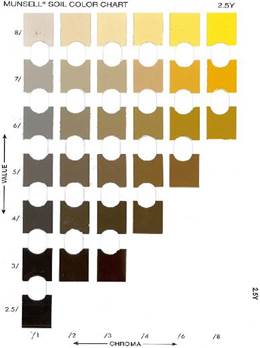
The Munsell soil-color charts (MSCCs) are derived from the Munsell space color and represent a part of the Munsell hue spectrum. There are several versions, but each is composed of a subset of charts representing a different hue in the Munsell space. Each chart has multiple color chips originating from the degrees of luminance and purity of color known as value and chroma. Figure 1 shows one of the seven charts of the USA2000 version.
The transformation from RGB to Munsell color space is a relevant issue for different tasks that require applying the conversion to images taken from traditional cameras or smartphones. For example, in Edaphology, the transformation of a sample soil image to the Munsell soil-color charts (MSCCs) is required to identify the taxonomy and characteristics of the soil in geographical areas (Sánchez-Marañón et al., 2005; Domínguez Soto et al., 2018; Ibáñez-Asensio et al., 2013). Likewise, in archaeology, Munsell soil-color charts (MSCCs) are useful for identifying organic materials, soil proles, rock materials, textiles, metals, colored glasses, paintings, and the artifacts retrieved (Milotta et al., 2017; Milotta et al., 2018a). In addition, the transformation from RGB color space to Munsell soil-color charts (MSCCs) could be used to identify skin, hair, and eyes in Anthropology, Criminology, Pathology, and Forensic Medicine (Munsell Soil Color Charts, 2000). Some studies have aimed to build a model to predict the value, chroma, and hue of MSCCs from RGB images (Pegalajar et al., 2018; Stanco et al., 2011; Milotta et al., 2017, Milotta et al., 2018a, Milotta et al., 2020) to solve the imprecision of professionals (Edaphologists and Archaeologists) when predicting value, chroma, and hue based on MSCCs. This paper is in the same line as those investigations. The goal is to find a model to accurately predict the HVC of MSCCs from images in RGB space captured in an uncontrolled environment. It means in the field without controlling the illumination, inclination, and position of the images.
The challenge to obtain an accurate model with images taken in an uncontrolled environment lies in the fact that two photos captured with the same device will have different RGB values due to the lighting exposed or other conditions such as the camera inclination or the distance between the camera and the object.
Related work
ANN to Move From RGB to Another Space Color
Some studies experimented with artificial neural networks to predict a color space values from images represented in RGB. For example, León et al. (2006) proved different methods to move from RGB to L*a*b. These methods are the following: a) a transformation based on a linear function; b) a quadratic model, which considers the influence of the square of the variables (R, G, B) on the estimate of the values L*a*b; c) a direct model that, in the first step, carries out the RGB to XYZ transformation and, in the second step, the XYZ to L*a*b; d) a model that adds the gamma correction to the previous one; e) finally, a model based on artificial neural networks. The best prediction was obtained with an ANN of three layers.
The first layer took the RGB values of a pixel as input, the second was a hidden layer with three neurons, and the last gave the L, a, b values as output. Another example is the transformation from Munsell space to CIE XYZ through an ANN with four nodes (Viscarra-Rossel et al., 2006).
The Transformation From RGB to Munsell Space
In Gómez-Robledo et al., (2013), an application to transform an RGB soil sample image taken from a smartphone into Munsell notation was built. The images were taken under controlled conditions of lighting and position. Polynomial transformations using the pseudo-inversion method were implemented to convert one space into another.
Unlike Gómez-Robledo et al., (2013), some researchers have created an application named ARCA (Milotta et al., 2017, Milotta et al., 2018a, Milotta et al., 2018b) to predict hue, value, and chroma of MSCCs from images taken in an uncontrolled environment. For the prediction, they used the Centore transformation (Centore, 2011) and the application of the discretization to round the values predicted.
The study of Pegalajar et al., (2018) was the first one, as far as we know, that applied machine learning to predict the HVC values from RGB images. In their system, three artificial neural networks received Red, Green, and Blue mean values of an image as input, and one of them released the hue value as output; another one, the value; and the last one, the chroma value. In a second stage, the HVC predicted for each image was used for a fuzzy system to return the exact MSCC chips.
In a recent study by Milotta et al., (2020), a support vector classifier (SVC) was trained to classify images of MSCC chips taken in an uncontrolled environment to an HVC chip. The authors suggested applying deep learning techniques in future studies to improve the prediction.
Methodology
Data Generation
We used images of the MSCCs taken from Milotta et al. (2018b) for training and testing the model. The authors took photos of the Munsell soil-color charts from 2000 and 2009 versions in the most uncontrolled environment. We used only the hue charts that are common in both versions: 10R, 2.5YR, 5YR, 7.5YR, 10YR, 2.5Y, and 5Y.
The photos were taken in Tampa-Florida (GPS coordinates 28°03’ 47.9’’ N 82°24’ 40.9’’ W), from 10:30 a.m. to 12:30 p.m. on different days, under 12 different settings (Milotta et al., 2017), that come from:
Of all the images, only those that had the Gretag-Macbeth color checker were used, as shown in Figure 2, because we wanted to incorporate, in the learning model, information about changes in the illumination, using the B1, D1, and E1 Gretag-Macbeth color patches. These colors work as a white reference to track the changes in the illumination.
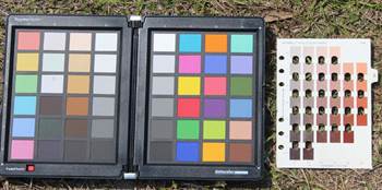
For the dataset preparation, we developed a tool to manually extract and label a piece of a sample of every chip along with the reference patches of the Gretag-Macbeth color checker. The sample images generated by the tool had a size of 8x8 pixels. In total, 78 pictures were used to create the complete dataset; this included the Munsell charts images from both available versions. After the chip and reference extraction, two approaches were implemented. The first one appended the reference samples to the chip image to train convolutional neural networks. Since most of the information came from the chip, the images were resized until the output image had approximately a 3:1 size relationship between chip and references, as shown in Figure 3. In total, we obtained 2856 images to train, validate and test the models.

The second approach permits training a feedforward neural network. In this case, a CSV file was generated for each chip of the dataset; each row in this file contained the ground truth HVC values of the chip, the average RGB values of the chip and the average RGB values of each B1, D1, and E1 reference.
In both cases, a division of 10% for testing, 20% for validation, and 70% for training was used. The partitions had the same image data for both the convolutional neural network and the feedforward neural network; this was done to have a common ground for comparison between the two approaches.
Proposed Models
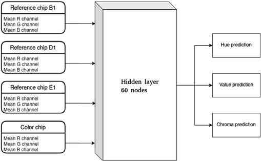
The feedforward neural network architecture for regression and classification was as follows:
The input consisted of twelve values, three of which correspond to the average of the R, G, and B values of each chip. Nine values were the average of the R, G, B of the reference blanks.
The input and output values were normalized from 0 to 1.
A hidden layer with 60 nodes and a sigmoid activation function.
The output layers were three for the regression nets: hue, value, and chroma. In the case of classification, we developed three nets with different outputs. The hue net had seven outputs, one for each possible hue. The Value net had seven outputs. The chroma net had six outputs.
The optimization function is the combined mean square error of hue, value, and chroma in the regression nets and the cross-entropy error in the classification nets. The optimization algorithm is Levenberg-Marquardt, which combines the steepest gradient descent and the Gauss-Newton algorithms (Afifi & Brown, 2019), with a maximum of 1000 epochs and a stop criterion, which consists of stopping after 50 epochs without improvement in the validation sample's loss function. The regression model gives numerical predictions of hue, value, and chroma. However, we need to classify each output in one of the 248 possible value combinations of hue, value, and chroma (chips) of our Munsell Charts. Therefore, the Euclidean distance was used with the regression net predictions to find the most similar combination (chip) from all HVC possible values. We also applied a convolutional architecture for regression and classification. The objective was to develop a lightweight model that could complete the task successfully.
The architecture of the model is as follows:
Note: derived from research.
Figure 4 Feedforward Neural Network. Note. For classification, we developed three nets with different outputs. The Hue and Value net had seven outputs, one for each possible value. The chroma net had six output.
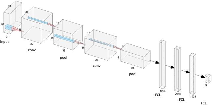
Input: The image generated from the chip and the white of reference, as in Figure 2, but amplified to 40x40 pixels in order to have a larger and wider image for the convolution process (Input).
2D convolution, out_channels=32, kernel_size=5, stride=1, ReLU activation function, batch normalization and average pooling (conv_1+pool_1 in Figure 5).
2D convolution, out_channels=64, kernel_size=3, stride=1, ReLU activation function, batch normalization and average pooling (conv_2+pool_2, in Figure 5).
Fully connected Layer, out_channels=4096, ReLU activation function (FCL_1, in Figure 5).
Fully connected Layer, out_channels=2048, ReLU activation function (FCL_2, in Figure 5).
Fully connected Layer, out_channels=1024, Sigmoid for regression and softmax for classification. (FCL_3, in Figure 5)
Output: Three outputs for the regression nets: hue, value, and chroma. In the case of classification, we developed three nets with different outputs. The Hue net had seven outputs, one for each possible hue. The Value net had seven outputs. The chroma net had six outputs.
The mean absolute error was used as the loss function for regression and cross-entropy for the classification nets. Adam was
Note: derived from research.
Note. For classification, we developed three nets with different outputs. The Hue and Value net had seven outputs, one for each possible value. The chroma net had six output.
the optimizer, with a learning rate and weight decay value of 0.0001. The weights were updated only when the validation accuracy of a specific epoch surpassed the best validation accuracy reported to the moment or a base accuracy value of 50%. The Euclidean distance was used with the regression net predictions to find the most similar chip from all HVC possible values. Thus, the numerical values were converted to classification values. The models were implemented in Python using Keras and executed in Google Colaboratory.
Analysis and Results
For the testing sample, Table 1 shows the percentage of chips classified correctly, the correct percentage classification of hue, value, and chroma, and the CIEDE2000 distance between prediction and ground truth for the different models. This distance was proposed to determine the color differences between the two images.
In order to have a baseline, the Transformation of Centore (Centore, 2011) was applied to the chips' RGB mean values for the prediction of the HVC values, similar to Stanco et al. (2011). After that, we used a discretization to round the values obtained from the transformation. This methodology achieved 61.2% accuracy, and the mean CIEDE2000 was 8.16, with a standard deviation of 3.64. Almost all the models generated surpassed the Accuracy of the Centore's Transformation; the only exception was the feedforward for regression without the whites of references (FFN_WWF). This result shows the importance of including information in the models about the illumination changes.
The best approach was the convolutional neural networks for classification (CNN_cla) with approximately 93% of total accuracy (it consisted of three CNN). The cases classified incorrectly with this approach had a CIEDE2000 average of 0.27 and a standard deviation of 1.06, which were lesser than the method of Centore (Centore, 2011). According to Yang, Ming, and Yu (2012), a distance between 0 and 0.5 is hardly perceived. We developed three models in this approach instead of one because there were not enough images to build a classification model with 7*7*6 outputs.
Conclusions
The transformation from RGB to Munsell color space is a relevant issue for different tasks that require applying the conversion to images taken from traditional cameras or smartphones. In this paper, we proposed different learning models to predict the hue, value, and chroma in the Munsell soil-color charts (MSCCs) from RGB images. The best approach surpasses the Transformation of Centore (Centore, 2011) and shows 93.0% of accuracy. This approach is based on three convolutional neural networks that used images to combine the chip and whites of references as input to track the changes in the illumination. Although this percentage is promising, the model should be tested with real images at different applications, such as soil real images, to classify the soil color.
Furthermore, future research should emphasize improving the accuracy and the construction of a device-independent model to apply in images taken from other devices. An alternative to accomplish this task is the application of recent DNN that estimates the illuminant of an image independent of the sensor device RGB response to the scene's illumination (Hernandez-Juarez et al., 2020; Marquardt, 1963). These DNN could be applied, in the first stage, to the Munsell images to neutralize the illuminant effect, independent of the sensor's device. In the second stage, the neutralized images could be used to train an independent device model for HVC prediction.
Table 1 Accuracy and CIEDE200 distance of the models.
| Model | Total | Hue | Value | Chroma | Mean_ CIEDE | Sd_CIEDE |
| Centore | 61.2% | 71.3% | 94.1% | 91.6% | 8.16 | 3.64 |
| FFN_WWF | 23.4% | 55.6% | 81.8% | 49.7% | 4.15 | 3.40 |
| FFN_reg | 87.1% | 95.5% | 99.0% | 90.2% | 0.52 | 1.40 |
| FFN12_cla | 76.2% | 94.1% | 96.2% | 83.9% | 1.08 | 2.06 |
| CNN_reg | 82.2% | 87.0% | 98.1% | 93.7% | 0.57 | 1.41 |
| CNN_cla | 92.9% | 99.3% | 98.9% | 94.4% | 0.27 | 1.06 |
FFN_WWF= feedforward without white of reference, FFN_reg= feedforward for regression, FFN_cla= feedforward for classification, CNN_reg Convolutional Neural Network for regression, CNN_cla= Convolutional Neural Networks for classification. The best result is in bold.
Note: derived from research.

