


 Spanish (pdf)
 Article in xml format
 Article references
 Send this article by e-mail
 Cited by SciELO
  Similars in
SciELO
Similars in
SciELO 
 Permalink
I. INTRODUCTION
The microeconomic analysis of fuel demand has long been considered a subject of importance both because of its effects on economic development and due to its environmental impact (1). Along this line of reasoning, fundamental research questions have been related to the price effect on fuel demand and the causal relations between energy demand and economic output, particularly any indirect effects of energy price constraints on output. Similar approaches have been adopted to the impacts of infrastructure investment and transport costs on development (2).
Fuel demand in Costa Rica has been regularly studied over the last three decades. Generally, previous research can be classified into one of two categories: academic research examining price and income effects, motivated by the environmental impacts of fuel consumption (3), (4), (5), and government analysis to inform energy sector planning (6), (7) —of strategic importance, given the State control of fuel imports and electricity production in Costa Rica. Most previous research has resulted in elasticity estimates derived from aggregate demand using time series econometrics (3), (4), (6), (7). Blackman et al. (5) are an exception: they used household survey data to conclude the tax on gasoline is progressive and the tax on diesel, regressive in Costa Rica. More recently, Godínez-Zamora et al. (8) generated scenarios for deep decarbonization in Costa Rica for the energy and transport sector, based on stakeholder input, which they subsequently simulated with the OSeMOSYS model; they found out greenhouse gas emissions could be reduced by up to 87 % of the baseline by a combination of modal shift, technology, and demand management.
Elasticities were estimated by Singh and Vargas (3) for gasoline (-0.33 of price and 0.47 of income) and for diesel (-0,20 of price and 0,33 of income) demand during 1972-1992, after controlling for vehicle ownership. Adamson (4) used a time series of 1957-1996 to estimate, for gasoline and diesel, elasticities of price (-0.26 and -0.18, respectively) and income (1.41 and 0.88, respectively). Neither Singh and Vargas (3) nor Adamson (4) found significant cross elasticities between fuel prices. Leiva (7), in his most recent energy elasticity estimates for Costa Rica, used data of 1984-2007 to calculate price and income elasticities for diesel demand (-0.14 and 0.97, respectively) and premium gasoline (-1.03 and 1.29, respectively); regular gasoline estimates only included income elasticity (1.05) because the price elasticity was found to be positive, likely because of substitution of premium gasoline during high price periods.
This paper reports a time series analysis of fuel demand, Gross National Income (GNI) per capita (as a proxy variable for household income), and gasoline price. The stationarity of all-time series was explored, followed by cointegration of all series with a common integration order. Granger causality was determined. A vector autoregression (VAR) model is reported to understand the magnitude, sign, and significance of determinants.
The analysis completed in this paper extends previous work on aggregate fuel demand in two directions. Firstly, it makes use of longer time series of fuel demand (for the 1965-2019 period, encompassing 55 years), this allows for more rigorous modeling of serial correlation than previous work (3), (4), (7). Secondly, it applies a VAR, which allows for endogenizing all variables. In particular, the developed model extends previous work by considering income as potentially endogenous –unlike models reported in (3), (4), (7), all of which assumed exogeneity of price, income, and vehicle ownership.
II. METHODOLOGY
A. Data on gasoline demand and price, vehicle ownership, and income in Costa Rica, 1965-2019
Following previous work and, more generally, the literature on the relation between transport demand and income (e.g. (9), (10)), a series of equations were proposed to explain the relationship between transport activity (fuel demand and vehicle ownership), fuel price (which is also a good proxy for direct transport costs), and income, as represented by Gross National Income per capita:
 (1)
(1)
 (2)
(2)
 (3)
(3)
 (4)
(4)
with QTt the yearly fuel demand per capita (gasoline or diesel), Fleett the number of registered vehicles per capita, Pt the fuel price per liter, and INDt the Gross National Income per capita; further, r is the optimal amount of lags (selected to maximize a set of information criteria), and μi,t the random error term. The model formed by this set of equations was estimated for annual data of Costa Rica, 1965-2019. 1 Gasoline price and Gross National Income per capita are expressed in real terms. Models were estimated separately for gasoline and diesel. Fleett was defined by the number of cars to model gasoline demand, as this is the fuel mostly used by private vehicles; for diesel demand, the sum of trucks and buses was used due to their role in consuming most diesel fuel for transport in Costa Rica (data on the number of vehicles per fuel is not available in national statistics, requiring the use of these proxy variables). All data series were transformed into natural logarithms.
TABLE I DESCRIPTIVE STATISTICS OF ANALYZED TIME SERIES 2
| Variable | Mean | Standard deviation | Minimum | Maximum |
| Gasoline demand per capita (m3 per person) | 141,9 | 68,8 | 54,0 | 266,4 |
| Diesel demand per capita (m3 per person) | 193,9 | 50,7 | 93,9 | 285,9 |
| Registered cars per capita (vehicles per 1000 persons) | 78,2 | 54,0 | 15,1 | 193,8 |
| Registered trucks and buses per capita (vehicles per 1000 persons) | 32,7 | 31,1 | 8,1 | 51,0 |
| Gasoline price (colones/litre) | 617,3 | 200,0 | 324,0 | 1111,1 |
| Diesel price (colones/litre) | 439,5 | 206,5 | 125,6 | 880,9 |
| Gross National Income per capita (USD$ per person) | 5645 | 1914 | 3023,0 | 9557,0 |
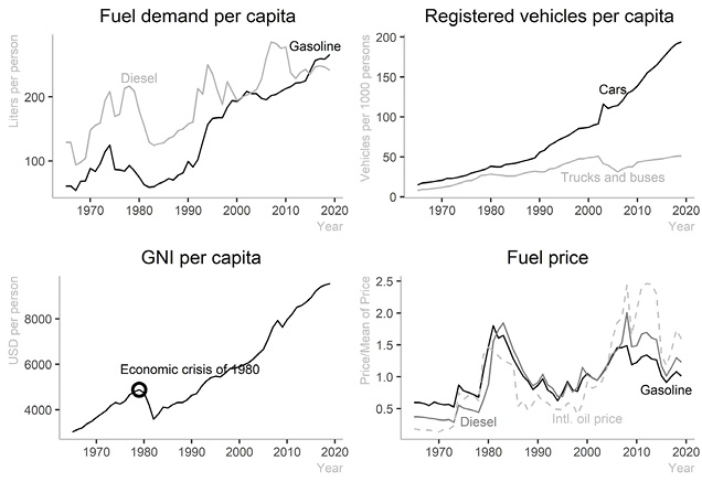
Fig. 1. Fig. 1. Trends of fuel demand per capita, total registered vehicles per capita, fuel price, and Gross National Income per capita (1965-2019).
Based on the literature review, one may expect: (a) Gross National Income per capita and fuel demand per capita to be caused (in the sense of Granger) by other variables, (b) price to be exogenous, i.e., not caused by other variables, (c) price should be a negative determinant of both fuel demand and Gross National Income per capita, and (d) Gross National Income per capita to be a positive determinant of gasoline demand.
Descriptive statistics and trends of the time series are reported in TABLE I and Fig. 1. Fuel demand, for both gasoline and diesel, shows an overall increasing trend with fluctuations. Dispersion in the data is greater for gasoline demand (a coefficient of variation of 0.48) than for diesel (coefficient of variation of 0.26). Similarly, the ratio of maximum to minimum values is greater for gasoline demand (nearly five) than for diesel (three). Two other time series show an overall increasing trend but with smoother fluctuations: Gross National Income (which clearly display a dip in 1980, a year of sharp economic crisis in Central America) and registered trucks and buses; the latter exhibits a large dispersion (a coefficient of variation of 0.95) for trucks and buses, there is in Fig. 1 a relatively smooth increase from 1965 until the early 2000s, after which there is a decrease followed by an increase. On the contrary, the number of cars per capita shows a smooth increasing trend, with relatively large dispersion (coefficient of variation of 0.69) and a remarkable growth of over ten times over the 1965-2019 period.
The most likely exogenous time series, those of price, show larger fluctuations than other variables —and indeed one could argue they do not exhibit the increasing trend of fuel demand, registered vehicles per capita, and Gross National Income per capita. These fluctuations coincide with, and likely respond to, the mean price of oil in the international markets (Fig. 1). Additionally, it is also apparent diesel prices have been larger than the mean towards the end of the study period, specifically after 2008 when the subsidy to diesel price (in the form of a large price differential with gasoline) was substantially reduced. This also explains why the dispersion in the diesel price data is larger (coefficient of variation of 0.47) than in the gasoline price data (coefficient of variation of 0.32), albeit both are similar to each other and less than dispersion in international oil prices (coefficient of variation of 0.68).
B. Econometric strategy
The quantitative model exploring the endogeneity of the time series, proposed in subsection A, was developed in two stages. First, Granger causality between the time series was explored; second, the VAR model on first differences was estimated and discussed.
Granger causality is based on the transmission of information: in the sense of Granger, a time series, yt, is said to be caused by another time series, xt; if yt can be better predicted by considering the past of both yt and xt rather than only the past of yt (11). Formally, consider:
 (5)
(5)
 (6)
(6)
The hypothesis test H0: b1 = b2 = … = br = 0 vs. HA “not H0”, tests if xt does not cause yt (in the sense of Granger); similarly, the hypothesis test H0: d1 = d2 = … = dr = 0 vs. HA “not H0” tests if yt does not cause xt. Rejecting the null hypothesis implies the existence of Granger causality.
When time series have integration orders greater than 0, conventional Granger causality tests may present problems due to the inapplicability of conventional asymptotic theory (12). As noted by Todaro and Yamamoto (12), VAR models can be generated for known orders of integration or cointegration rank; however, (a) tests to determine their properties are limited when data have small samples and (b) often, as in the present paper, interest is not on forecasting but rather on the relations between variables themselves. Todaro and Yamamoto (12) suggested Granger causality should be tested on the levels of a VAR, regardless of integration order, but to control for the bias introduced by the use of levels with a greater number of lags: specifically, they proposed to determine the maximum integration order, I(k), of all time series in the model and to increase the amount of lags in the VAR by k. These results would be used to perform the Granger causality test; however, the k additional lags would not be included in the test itself.
Thus, the Granger causality tests applied to the set of time series described in subsection A were developed as follows: (1) the augmented Dicky-Fuller test was used to test for unit roots in each time series, from which their order of integration, I(k), was determined (these results are summarized in TABLE II); (2) the optimal lag, ro, to maximize a set of four information criteria was selected for a VAR model on the levels of all time series; (3) the VAR model was estimated with (ro+k) lags, and (4) a Wald test was performed considering only the coefficients of the first ro lags (i.e., with ((v-1)·ro) degrees of freedom, with v the number of variables in the model), to determine Granger causality (see TABLE III). As potential verification of Granger causality, cointegration between the data series was explored (TABLE IV), because cointegration implies causality, although the absence of cointegration does not necessarily reject it.
To further explore the causal determinants, a VAR model on differences to make the data stationary was reported in TABLE V. From it, the sign, significance, and magnitude of the relations between variables were explored.
III. RESULTS AND DISCUSSION
The development of dynamic time series models must begin by a characterization of the properties of the time series themselves, the most basic of which is their integration order. TABLE II summarizes the results of the augmented Dickey-Fuller tests, which are used to determine the existence of unit roots in the data.
TABLE II AUGMENTED DICKEY-FULLER TEST STATISTICS 3
| Variable | Level | First difference | ||
| Trend | Drift | Trend | Drift | |
| Gasoline demand per capita | -1.770 | -0.778 | -4.309* | -4.354* |
| Diesel demand per capita | -2.819 | -1.914 | -5.121* | -5.137* |
| Registered cars per capita | -2.357 | -1.191 | -6.098* | -5.987* |
| Registered trucks and buses per capita | -1.976 | -2.476 | -3.453+ | -3.116+ |
| Gasoline price | -2.292 | -2.258 | -5.094* | -5.069* |
| Diesel price | -2.035 | -1.822 | -4.562* | -4.571* |
| Gross National Income per capita | -2.402 | -0.569 | -5.138* | -5.190* |
* p < 0.01, + p < 0.05
The results from TABLE II clearly show (a) log-transformed levels of the variables considered are not stationary and (b) they are of integration order 1, i.e., their first difference is stationary (the weakest ADF test statistic corresponds to the trucks and buses time series, but it is still significant with p<0.05). On unit root testing, see Lütkepohl (13).
TABLE III was estimated using the Toda and Yamamoto (12) approach to Granger causality testing, i.e., estimating a VAR model on the levels of time series (despite the levels not being stationary per the results of TABLE II), and adding as many lags as the maximum order of integration of all-time series involved (in the present case, one additional lag, as all-time series were found to be of order 1). To estimate this VAR model on the levels, the number of lags was chosen by (1) maximizing a set of information criteria (which suggested 1 lag for both the gasoline and diesel models), (2) verifying the both models correspond to stable VAR processes, (3) revising if a greater number of lags might mitigate serial correlation in the error terms (specifically for the diesel model, serial correlation problems in the error term persists with 1 lag but increasing the number of lags exacerbates the problem). It is important to note that the VAR model for diesel demand excludes the number of registered vehicles (trucks and buses) because, regardless of the number of lags selected, the resulting models were not stable.
As can be seen in TABLE III, both gasoline and diesel demand are Granger caused by other time series, as well as Gross National Income per capita (in both models). Similarly, there is no causal effect on price, neither for gasoline nor for diesel, which is consistent with the relation of price with the international oil prices (see Fig. 1). In general, the hypothesized relations between income (Gross National Income per capita), fuel price, and fuel demand are supported by the model. However, it is noteworthy that the variable cars per capita is not caused by other potential determinants, in particular by the income proxy variable, as mode choice has been linked to household income (e.g. in origin/destination travel surveys, (14)).
TABLE III GRANGER CAUSALITY MODELS 4
| Dependent variable (effect) | Determinants (causes) | X2 (d.f.) | Prob. |
| Gasoline model | |||
| Gasoline demand per capita | Registered cars per capita, gasoline price, Gross National Income per capita | 36.155 (3)* | <0,001 |
| Registered cars per capita | Gasoline demand per capita, gasoline price, Gross National Income per capita | 2.072 (3) | 0.558 |
| Gasoline price | Gasoline demand per capita, registered cars per capita, Gross National Income per capita | 1.521 (3) | 0.677 |
| Gross National Income per capita | Gasoline demand per capita, registered cars per capita, gasoline price | 10.993 (3) + | 0.012 |
| Diesel model | |||
| Diesel demand per capita | Diesel price per capita, Gross National Income per capita | 7.932 (2) + | 0.019 |
| Diesel price | Diesel demand per capita, Gross National Income per capita | 2.016 (2) | 0.365 |
| Gross National Income per capita | Diesel demand per capita, diesel price | 10.994 (2)* | 0.004 |
* p < 0.01, + p < 0.05.
A combination of nonstationary series may be said to be stationary in which case they are called cointegrated and they share a common stochastic trend. Cointegration is evidence of Granger causality. The stationary linear combination may be interpreted as a long-run equilibrium (9). Cointegration, in sum, is an interesting property to explore if present in the data. To detect the existence of cointegration in the time series being analyzed, the Johansen cointegration test was performed (see Lütkepohl (13)). The results are reported in TABLE III. The Johansen test for cointegration may be specified as trace or maximum eigenvalue: for each type, the alternative hypothesis is different which may lead to slightly different results. TABLE IV reports the statistics for Johansen's test (for both the trace and eigenvalue versions of the test) and their probability.
The results of TABLE IV show hardly any cointegration exists between the time series: the Eigenvalue statistic for the gasoline fuel VAR model suggests the existence of one cointegration relation, but this is not confirmed by the trace statistics. Neither does the diesel fuel VAR model display any evidence of cointegration. It should be noted that estimating the (unreported) vector error correction model (VECM) for gasoline fuel does yield a significant long-run error correction term for gasoline demand and Gross National Income per capita as dependent variables, suggesting this to be the cointegrated time series. Yet this VECM sheds limited information on the relations between determinants: because the optimal VAR model is of lag 1, there are no short-run relations in the VECM, only the long-run error correction term (which, in turn, is only significant for two of four possible variables).
TABLE IV JOHANSEN COINTEGRATION TEST RESULTS
| Null hypothesis | Alternative hypothesis | Trace statistic (prob.) | Eigenvalue statistic (prob.) |
| Gasoline demand per capita, registered cars per capita, gasoline price, Gross National Income per capita | |||
| r ≤ 3 | r > 3 | 1.157 (0.282) | 1.157 (0.282) |
| r ≤ 2 | r > 2 | 7.789 (0.828) | 3.633 (0.887) |
| r ≤ 1 | r > 1 | 16.654 (0.673) | 11.863 (0.573) |
| r = 0 | r > 0 | 44.232 (0.104) | 27.579 (0.047) + |
| Diesel demand per capita, diesel price, Gross National Income per capita | |||
| r ≤ 2 | r > 2 | 0.006 (0.936) | 0.006 (0.936) |
| r ≤ 1 | r > 1 | 8.034 (0.469) | 8.028 (0.384) |
| r = 0 | r > 0 | 20.330 (0.412) | 12.296 (0.532) |
+ p < 0.05.
In order to analyze further evidence on these relations, and in light of the limitations of the VECM, the VAR model on first differences is reported in TABLE V for gasoline and diesel fuels.
TABLE V VAR MODELS ON FIRST DIFFERENCES OF GASOLINE AND DIESEL FUEL DEMAND
| Determinant (cause) | Gasoline models | Diesel models | |||||
| ΔGasoline demand | ΔPrice | ΔGNI | ΔFleet | ΔDiesel demand | ΔPrice | ΔGNI | |
| Intercept | 0.038* | -0.010 | 0.016* | 0.056* | -0.046 | 0.027 | 0.018* |
| ΔQTt-1 | -0.166 | 0.312 | -0.009 | -0.004 | -0.046 | 0.225 | -0.010 |
| ΔPt-1 | -0.401* | 0.162 | -0.102* | -0.037 | -0.236* | 0.120 | -0.100* |
| ΔGNIt-1 | 0.660+ | -0.232 | 0.349* | 0.100 | 0.456 | -0.462 | 0.253+ |
| ΔFleett-1 | -0.320 | 0.302 | -0.020 | -0.244+ | — | — | — |
| Adjusted R2 | 0.324 | <0.01 | 0.219 | 0.007 | 0.135 | <0.01 | 0.290 |
| f stat. | 7.241 | 0.718 | 4.637 | 1.094 | 3.703 | 0.463 | 8.085 |
| d.f. | 4 & 48 | 4 & 48 | 4 & 48 | 4 & 48 | 3 & 49 | 3 & 49 | 3 & 49 |
| Prob. | <0.001 | 0.584 | 0.003 | 0.371 | 0.018 | 0.709 | <0.001 |
* p < 0.01, + p < 0.05
The VAR models for both fuels confirm price as an exogenous determinant: no other variable in the system is a significant determinant of the first difference of either gasoline or diesel price. Furthermore, and perhaps more surprisingly, neither there are any significant determinants (save the intercept) of the first difference of cars per capita in the gasoline fuel VAR. These three equations (of gasoline price, diesel price, and fleet) all show adjusted coefficients of determinations lower than 0.01 and non-significant f statistics.
The first difference of Gross National Income per capita, in both VAR models, is clearly the variable most determined by others in the model: both the first lag of Gross National Income per capita and of price (as well as the intercept) were significant. Price presented a negative sign, Gross National Income a positive sign. Adjusted coefficients of determinations—for a model in first differences—are relatively large (over 0.20) and f statistics reject the null hypothesis that all coefficients are not different from 0. In sum, these results are in line with the theoretical expectations of the price mechanism: the available income grows in the long-run (which can be seem in Fig. 1) and high fuel prices reduce available income.
As for the gasoline demand, it is also generally in line with theoretical expectations: the model presents an adjusted coefficient of determination of 0.32 (the largest among all equations in both models), a large f statistic, and significant determinants for the first difference of price (negative) and Gross National Income per capita (positive). The only unexpected result is motorization (i.e., the first difference of cars per capita) was not a significant determinant of per capita gasoline demand.
Diesel demand in TABLE V is a much weaker model than gasoline demand, which also should be expected: the use of diesel is more concentrated on the less elastic freight and public transport. Indeed, previous results also coincide with the results of TABLE V in identifying diesel price and income elasticities as less than the corresponding elasticities for gasoline (3), (4), (7). Price is a significant determinant and negative of diesel per capita demand; unexpectedly, the income proxy Gross National Income per capita is not a statistically significant determinant.
The results reported in TABLE III and TABLE V, as already argued by Singh and Vargas (3), advocate for fuel taxes as effective instruments to reduce fuel consumption: an increase in fuel price, which may be induced by a tax, reduces per capita demand (as evidenced by the Granger causality of fuel demand and the negative, significant coefficients of price in the fuel demand models). Direct benefits of such taxation, in addition to carbon emissions reductions, include pollution abatement and related health benefits as well as time savings from decreased congestion (3). This effect is larger for gasoline and, thus, should have more limited impacts on public transport (the buses that supply it are dependent on diesel and, because of it, diesel price increase has been found to present regressive effects on income (5)) and on freight. Furthermore, it is also important to note that the lagged first difference of fuel demand is not a significant determinant of Gross National Income per capita (TABLE V); therefore, the transport and fuel demand constraints imposed by greater price should have limited repercussions on household income and prosperity.
Policy interventions on fuel demand require further analysis, as population and economic activity patterns in Costa Rica are greatly concentrated; indeed, data for spatio-temporal analysis is available (16) and its analysis may provide valuable insights into actionable policy. Specifically, the San José metropolitan region concentrated, in 2019, 56 % of gasoline demand 46 % of diesel demand (16); regional average household income in the Central Region (of which the San José metropolitan region is part) is also 1.19 times greater than the country average (17). Traffic congestion has also been found to be fundamentally centered in Costa Rica (18). In synthesis, a surcharge on fuel prices in the San José metropolitan region may have greater benefits and less distributional disadvantages, as the problems addressed by this traffic management strategy (i.e., an increase of transport costs via greater fuel price, particularly for private cars) are centralized there.
The analysis presented in this paper corresponds to a long time series of data —55 years, between 1965 and 2019. During this period, the Costa Rican economy has undergone various important changes that could have modified the relation between fuel demand, income, and price: population during this period more than tripled, during the 1980s, the economy diversified in response to the 1980 economic crisis, and the latest global financial crisis of 2007-2008 may also have drastically changed the trajectory of the Costa Rica economy. These changes may have introduced structural breaks into the time series, thus requiring controlling for them. The same argument could be made for the effects of the more recent COVID-19 pandemic, although there is insufficient data at present to account for it. The exploration of structural breaks is beyond the scope of the models reported in this paper, but it may be a fruitful area for further research (including a greater frequency of three-monthly data in lieu of annual time series).
IV. CONCLUSIONS
The analysis executed and reported in this paper shows evidence of causal relations between fuel demand and Gross National Income per capita. Time series including gasoline demand and Gross National Income per capita were found to present one cointegration relation (common stochastic trend) whereas the diesel fuel VAR resulted in no cointegration relations. Fuel price was found to be weakly exogenous.
The results of the developed models for gasoline and diesel demand are, on the whole, consistent with previous analysis of aggregate fuel demand in Costa Rica (3), (4), (6), (7). They provide confirmation of the potential for economic instruments for transport demand management; but they also provide cautionary signs necessary for the design and implementation of these policies. Fuel demand management is an attractive area for carbon mitigation, as most fuel consumption (of gasoline and diesel) is explained by transport demand (15), but it also may come with negative unforeseen effects on income (as implied by the negative and significant effect of fuel price on Gross National Income per capita in TABLE V).
Methodologically, the reported analysis extends previous work on fuel demand modeling in Costa Rica by endogenizing income (represented by Gross National Income per capita). This proved to be an important contribution for policy design, as negative effects of price on income were found to be statistically significant (however, there were no significant effects of fuel demand on Gross National Income). These conclusions may be conceptually evident; but the VAR model provides a quantitative methodological framework which may be used to assess the impacts of eventual taxation through, e.g., impulse response functions. More broadly, extensions of the model to other transport time series (e.g., air transport, traffic flows in key national roads) and the exploration of Granger causality with panel data structured per municipality (specifically, gasoline demand and its relationship with variables that characterize human settlements, such as number of jobs or population density) are promising fields for further research. The latter is particularly important because policy interventions can be tailored to focus on the San José metropolitan region, where the problems of traffic congestion are, and the benefits of fuel taxes should be concentrated.

