


 Spanish (pdf)
 Article in xml format
 Article references
 Send this article by e-mail
 Cited by SciELO
  Similars in
SciELO
Similars in
SciELO 
 Permalink
1. Introduction
Mexico has suffered significant degrees of disturbance in its natural ecosystems during the last five decades, due to the intensive exploitation of its natural resources. The complexity of such processes of change in land use and water bodies are determined by a network of complex interactions of socio-economic and environmental factors. Processes associated with the dynamics of change in land cover and land use are one of the main factors that determine the permanence, decline and extinction of different ecosystems and especially forests (Zhang et al., 2017). Thus, it is urgent to pay attention to the exploitation of environmental goods and services provided by different ecosystems. The primary sector, the rural environment and the evolution of economic activities keep straight relationship with changes in land use.
The critical approach to environmental sustainability has increased the interest in understanding the underlying causes of land use change. Numerous studies have been supported by the Land-Use and Land Cover Change (LUCC) project now called Global Land Program (GLP), contributing to the analysis of changes in the territory for more than a decade. Land use change is a very dynamic and complex process that relates natural and human systems. It has a direct impact on soil, water and the atmosphere and is directly related to several environmental problems of global importance (Meyer & Turner, 1994). Large-scale deforestations and subsequent transformations of agricultural land in the tropics are examples of extensive land use change with strong impacts on biodiversity (Lambin et al., 2003).
The impact of land use and land cover change on ecosystem health is one of the most important issues in land and ecosystem research (Deng et al., 2013; Leh et al., 2013; Newbold et al., 2015). Several studies have demonstrated the usefulness of methods, techniques and tools to analyze, evaluate and quantify the patterns of change, in order to understand their driving forces and depict their environmental and socioeconomic impacts (Darvishi et al., 2020; Homer et al., 2020; Matsa et al., 2020; Naikoo et al., 2020; Schürmann et al., 2020). In Mexico, is remarkable the work done on the evaluation and modelling of land use and cover change by Bonilla-Moheno & Aide (2020), Calzada et al., (2018), Hernández-Guzmán et al., (2018) and Mendoza-Ponce et al. (2018).
Several methods and approaches have been used to describe the nature and intensity of land use change. The use of quantitative methods to evaluate land use and cover changes have been described (Abreu & Ralha, 2018; Amadou et al., 2018; Li et al., 2020; Liu et al., 2020; Müller-Hansen et al., 2019). Linear regression has been used to measure the dynamics of vegetation (Abel et al., 2019), to estimate areas cultivation of rice and their yield (Chandra Paul et al., 2020), and to explore the factors influencing the production of agricultural charge (Dhulipala & Patil, 2020). Logistic regression was applied to determine the dynamics of forest cover (Bera et al., 2020; Saha, et al., 2020) and in studies of urban land use change (Cao et al., 2020). The development and advancement of geotechnologies such as GIS, has improved the efficiency of the study of land use changes (Prashar et al., 2013). Currently, GIS technology has contributed to the elaboration of descriptive, explanatory and simulation models, where spatial analysis techniques are used to understand and forecast the changes in land use that have occurred in the territory. The analysis of the change matrix to identify systematic signals within a change pattern has been proposed as model to describe the magnitude and trend of land use change at a geographic landscape from a statistical point of view (Pineda, 2010).
Implementation of spatial analysis in a GIS environment has improved the perception of geography, as space science, from a theoretical perspective, and as an applied science to organize the territory (Fuenzalida et al., 2015). However, most studies in land use and vegetation in Mexico analyze only the total change and do not search in deep for the net change, exchanges and transitions occurring between land use categories. The change matrix is not deeply examined; most times, only transition matrices are obtained, and annual change rates and total areas compared at times t1 and t2. Only occasionally the gains, losses and persistence in the landscape are calculated and interpreted. Thus, it is important to determine the magnitude of the changes that have occurred in vegetation, and waterbodies at Nayarit State, using methods and techniques that yield precise and detailed information regarding change processes in the landscape.
The aim of this research is to analyze and quantify the spatial and temporal trends of changes in land use, vegetation and water bodies, by calculating the losses, gains, net change, exchange and total change of each of the land use categories at Nayarit State, Mexico, 1993-2014.
2. Methods
2.1 Study area
The state of Nayarit, Mexico is located in the western portion of the country, between 20° 36 12 and 23° 05 04 in the north latitude and 103° 4315 and 105 ° 4537 of west longitude (Figure 1). Its surface occupies near 27 836 square kilometers. Although the archipelagos of the Islas Marías, las Marietas and Isla Isabel are part of the State, they were not considered in this study.
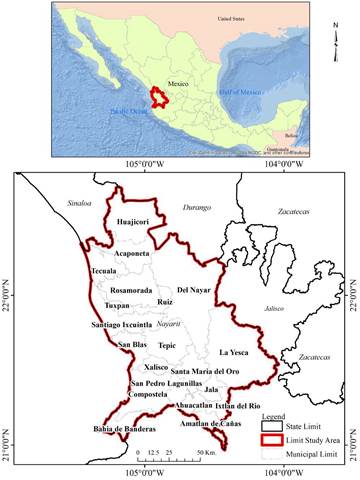
Source: Author, based on Marco Geoestadístico Nacional, 2017.
Figure 1 Map of the state of Nayarit, Mexico.
Its total population is 1,235,456 persons registered in the 2020 census (INEGI, 2021); 612,278 men and 623,178 women. Being one of the states with less inhabitants (place 29 out of 32) in the country. The predominant land uses are forests, oak, pine, mountain mesophyll communities, as well as associations with other types of plant cover (pine-oak, oak-pine). Considering their structures, there are medium sub deciduous forest, low deciduous forest, and low thorny shrubs, and several associations between these communities. There are also induced and cultivated grasslands growing on the coastal plains, along with mangroves, palm groves, savanna like vegetation, tular, popal, coastal dune vegetation, and halophilic and hydrophilic vegetation.
This state territory is a transition area of terrestrial ecosystems and marine ecosystems, it contains tributaries of rivers and streams, producing a mixture of fresh water and water of sea in this area, making it optimal for aquaculture. Besides, in this area of the Marismas Nacionales, aquaculture is allowed in the corresponding land management plan (Ponce-Palafox, 2015).
2.2 Data sources
As a reference base, two vectorial maps of land use and vegetation at scale 1: 250,000 in digital format (INEGI series II and series VI) were used. Series II map was elaborated from the visual interpretation of mosaics of satellite imagery obtained with the Thematic Mapper sensor (LANDSAT TM), acquired in 1993 with a spatial resolution of 50 m per-pixel. This map was modified by the National Institute of Ecology (INE), and according to Velázquez et al. (2002), has a level of precision and accuracy of 95%. Serie VI map was derived based as an update from V series map, made with photointerpretation techniques on multispectral satellite images (LANDSAT TM8) of 2014, with spatial resolution of 30 m per-pixel. Its quality was validated by the digital information standard of the National Statistical and Geographic Information System (INEGI, 2018). To process these maps, the date of acquisition of the imagery is considered, instead of the publication date of the map and in both cases the layer of aquaculture use (polygons of shrimp farms) was added to have a comparable vector information. Due to the process of map generation (photo interpretation) these maps are not error free, however both maps were verified by and intense field verifications. Besides considering the area extent, the scale of the data and the level of detail of the categories analyzed, the possibility of thematic and geometric errors of the coverage is minimal.
2.3 Map Processing and analysis
Map pre-processing included a preliminary review of previous categories in the study area. 18 land use classes were considered, and a common legend was elaborated so that the maps were comparable (Moreno & Chuvieco, 2009). Such legend reduced the differences in the definitions of class and type of vegetation, facilitating the comparison between products. Corresponding databases for each map were reclassified and homogenized. Topological vector correction was performed in order to relocate error and missing polygons and thematic standardization and filling of the database issues were solved. Both maps were reprojected to Universal Transverse Mercator coordinate system (Datum ITRF-92) and rasterized (1686 columns by 2196 rows). Star and Estes (1990) cited by Bosque (1997) suggested that the grid base size should be half the length than the smaller dimension needed to represent all the existing categories in reality. Considering this, a grid of 125 X 125 m was generated.
2.4 Methodological framework
Location and quantification of land use changes was done by cartographic overlaid of maps corresponding to before and after maps, and the estimation of a matrix of changes, generating maps and change tables that allow identifying the magnitude and spatial distribution of the change dynamics (Dupuy et al., 2007). Besides, in this study, losses, gains, net changes, total changes and exchanges between categories were calculated using the method by Pontius et al. (2004). It is important to note that the cartographic information is compatible, that is, they have the same area, scale and cartographic projection and comparable since they use the same legend or equivalence in the categories.
2.5 Analysis of the dynamics of land use, vegetation and water bodies
The analysis of change processes within each category is based on the matrix of changes (Table 1). The rows of the categories show time1 (t1) and the columns show time2 (t2). Additional column on the right indicates the proportion experiencing a gross loss of category i between time1 and time2. The additional row at the bottom indicates the proportion experiencing a gross gain of category j between time1 and time2. The diagonal shows the total amount of the stable class between dates, while the transitions of the classes between time1 and time2 are outside the diagonal.
Table 1 Matrix of changes to compare two maps of different times.
| Time 2 | Total time 1 | Losses | ||||
|---|---|---|---|---|---|---|
| Category 1 | Category 2 | Category 3 | Category 4 | |||
| Time 1 | ||||||
| Category 1 | P11 | P12 | P13 | P14 | P1+ | P1+ P11 |
| Category 2 | P21 | P22 | P23 | P24 | P2+ | P2+ P22 |
| Category 3 | P31 | P32 | P33 | P34 | P3+ | P3+ P33 |
| Category 4 | P 41 | P 42 | P 43 | P 44 | P4+ | P4+ P44 |
| Total time 2 | P+1 | P+2 | P+3 | P+4 | 1 | |
| Gains | P+1 P11 | P+2 P22 | P+3 P33 | P+4 P44 |
Source: Pontius et al., (2004).
With the information from the change matrix, the gain (Gij) was calculated, which is the difference between the total column of time2 (P+ j) and the persistence (Pjj) (expr. 1).
Gij = P+j Pij (1)
The loss (Lij) denotes the difference between the total row of time 1 (Pj+) and the persistence (Pjj), (expr. 2).
Lij = Pj+ Pij (2)
To calculate the total change for each category (Cj) it is established as the sum of the net change (Dj) and the exchange (Sj), or, the sum of the gains and losses (expr. 3).
Cj = Dj + Sj (3)
The exchange between categories (Sj) is calculated as twice the minimum value of gains and losses (expr. 4).
Sj 2 X MIN (Pj+ Pjj, P+j Pjj) (4)
The net change is defined as the absolute value of the difference between the gains and losses of each category (expr. 5).
Dj = |Lij Gij| (5)
To calculate the losses, gains, persistence, exchange and net change for each category the results of CROSSTAB command were exported to Excel, to convert cell units to hectares multiplying by the cell size (125 m2) and to calculate percentages.
3. Results
3.1 Analysis of the dynamics of land use and cover changes, vegetation and water bodies
In this study, 18 land cover categories were analyzed for the year 1993 (a) and 2014 (b) (Figure 2). In 1993, the low forest areas accounted for 20.82% of the total state coverage, while agriculture covered 18.17%. Similarly, the mixed forest (pine-oak forest and oak-pine) had 17.00% followed by the oak forest with the 16.98%, whereas the medium forest covered 14.85%, and water bodies occupied 1.63%. In 2014, agriculture increased its surface area and exceeded 22.14% of the state territory. The mixed forest comprised 19.13%, the medium forest occupied 15.05%, the low forest accounted for 13.76%, and the share of oak forests decreased to 12.11 %. Finally, water bodies occupied 1.91%.
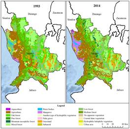
Source: INEGI Land use and vegetation mapping 1993 and 2014.
Figure 2 Land use and cover change in 1993 (a) and 2014 (b) at the vegetation type level.
According to the observed patterns, changes occurring within each category at Nayarit state are described and quantified. (Table 2) shows a summary of the matrix of changes in hectares and in percentages of the losses, gains, net change, exchange and total change of each of the analyzed categories. This makes it possible to clearly distinguish a net change from a total change, since the latter hides the exchanges that take place between categories. During the study period and at the coverage type level, the total change affected 2,783,572.50 ha. 58.06%, did not experience any change, while 41.94% presented some change in land cover, of which 15.42% denotes exchanges between the categories and 26.52% corresponds to a net change.
The real values of the change between 1993 and 2014 were obtained by means of the equation of the total change (expr. 3) that, unlike the net change (expr. 5), made possible to estimate the transitions between categories. In this regard, it should be noted that, if a category had gains and losses of the same magnitude, then net change would be equal to zero. Agriculture extended over an area of 505,767.3 ha in 1993, while for 2014, it increased to 616,147.2 ha. There was an increase of 110,380.00 ha, during a period of 21 years.
The increase in the mountain mesophilic forest stands shows a gain of 58,843.25 ha, considering a recovery of the forest cover, mainly at the municipalities of Del Nayar (22,611 ha) and Huajicori (16,899 ha). Another coverage with significant gains is mixed forests with 194,123.50 ha, mainly in the municipalities of Del Nayar (75,784 ha), La Yesca (41,787 ha) and, to a lesser extent Santa María del Oro (20,425 ha). The recovery of the mangroves is considerable showing a gain of 86,812.75 ha, which is most evident in the municipalities of Santiago Ixcuintla (34,718 ha), Rosamorada (21,667) ha and Tecuala (18,041 ha).
With regard to the loss of vegetation, low forest lost 287,422.75 ha, classified as a disturbance process. The municipality of Del Nayar has had the greatest alteration with 48,330 ha, followed by Santiago Ixcuintla with 38,081 ha and Huajicori with 30,316 ha. Oak forests lost almost half of its coverage (286,515.00 ha). This was recorded in the municipality of Del Nayar with 103,748 ha, La Yesca with 43, 784 and Huajicori with 33,073 ha. Halophilic and hydrophilic vegetation also suffered considerable losses (37,202.75 ha); this occurred more frequently in the municipality of Tecuala (15,700 ha), as well as in the municipalities of Santiago Ixcuintla (6,767) ha and Rosamorada (6,281 ha).
Table 2 Summary of the matrix of changes at the level of vegetation type (hectares and percentage).
| Total 1993 | Total 2014 | Gains | Losses | Total change | Exchanges | Net change | ||||||||
|---|---|---|---|---|---|---|---|---|---|---|---|---|---|---|
| ha. | % | ha. | % | ha. | % | ha. | % | ha. | % | ha. | % | ha. | % | |
| ACUI | 4096.8 | 0.15 | 9297.25 | 0.33 | 5291.50 | 0.19 | 91.00 | 0.00 | 5382.50 | 0.19 | 5200.50 | 0.01 | 182.00 | 0.19 |
| AGRI | 505767.3 | 18.17 | 616147.25 | 22.14 | 227096.00 | 8.16 | 116716.00 | 4.19 | 343812.00 | 12.35 | 110380.00 | 8.39 | 233432.00 | 3.97 |
| BENC | 472724.8 | 16.98 | 337187.25 | 12.11 | 150977.50 | 5.42 | 286515.00 | 10.29 | 437492.50 | 15.72 | 135537.50 | 10.85 | 301955.00 | 4.87 |
| BPIN | 6708.8 | 0.24 | 16482.50 | 0.59 | 13596.75 | 0.49 | 3823.00 | 0.14 | 17419.75 | 0.63 | 9773.75 | 0.27 | 7646.00 | 0.35 |
| BMM | 2057.3 | 0.07 | 60260.50 | 2.16 | 58843.25 | 2.11 | 640.00 | 0.02 | 59483.25 | 2.14 | 58203.25 | 0.05 | 1280.00 | 2.09 |
| BMIX | 473243.3 | 17.00 | 532600.25 | 19.13 | 194123.50 | 6.97 | 134766.50 | 4.84 | 328890.00 | 11.82 | 59357.00 | 9.68 | 269533.00 | 2.13 |
| CA | 45289.3 | 1.63 | 53092.00 | 1.91 | 12174.50 | 0.44 | 4371.75 | 0.16 | 16546.25 | 0.59 | 7802.75 | 0.31 | 8743.50 | 0.28 |
| MAN | 17819.0 | 0.64 | 98139.25 | 3.53 | 86812.75 | 3.12 | 6492.50 | 0.23 | 93305.25 | 3.35 | 80320.25 | 0.47 | 12985.00 | 2.89 |
| OTV | 87.3 | 0.00 | 7907.25 | 0.28 | 7830.50 | 0.28 | 10.50 | 0.00 | 7841.00 | 0.28 | 7820.00 | 0.00 | 21.00 | 0.28 |
| PAL | 5712.5 | 0.21 | 3605.25 | 0.13 | 2081.00 | 0.07 | 4188.25 | 0.15 | 6269.25 | 0.23 | 2107.25 | 0.15 | 4162.00 | 0.08 |
| PAS | 188672.5 | 6.78 | 184483.75 | 6.63 | 112744.75 | 4.05 | 116933.50 | 4.20 | 229678.25 | 8.25 | 4188.75 | 8.10 | 225489.50 | 0.15 |
| SAB | 6742.0 | 0.24 | 13785.00 | 0.50 | 12529.50 | 0.45 | 5486.50 | 0.20 | 18016.00 | 0.65 | 7043.00 | 0.39 | 10973.00 | 0.25 |
| SB | 579529.8 | 20.82 | 382925.00 | 13.76 | 90818.00 | 3.26 | 287422.75 | 10.33 | 378240.75 | 13.59 | 196604.75 | 6.53 | 181636.00 | 7.06 |
| SM | 413236.0 | 14.85 | 419029.50 | 15.05 | 166691.00 | 5.99 | 160897.50 | 5.78 | 327588.50 | 11.77 | 5793.50 | 11.56 | 321795.00 | 0.21 |
| SINVA | 222.0 | 0.01 | 4184.75 | 0.15 | 4184.75 | 0.15 | 222.00 | 0.01 | 4406.75 | 0.16 | 3962.75 | 0.02 | 444.00 | 0.14 |
| VDC | 861.0 | 0.03 | 1107.00 | 0.04 | 392.75 | 0.01 | 146.75 | 0.01 | 539.50 | 0.02 | 246.00 | 0.01 | 293.50 | 0.01 |
| VHH | 45805.0 | 1.65 | 15122.25 | 0.54 | 6520.00 | 0.23 | 37202.75 | 1.34 | 43722.75 | 1.57 | 30682.75 | 0.47 | 13040.00 | 1.10 |
| ZU | 14998.3 | 0.54 | 28216.50 | 1.01 | 14780.75 | 0.53 | 1562.50 | 0.06 | 16343.25 | 0.59 | 13218.25 | 0.11 | 3125.00 | 0.47 |
| Total | 2783572.50 | 100.00 | 2783572.50 | 100.00 | 1167488.75 | 41.94 | 1167488.75 | 41.94 | 1167488.75 | 41.94 | 369121.00 | 15.42 | 798367.75 | 26.52 |
Categorys: ACUI, aquaculture; AGRI, agriculture; BENC, oak forest; BPIN, pine forest; BMM, mountain mesophilic forest; BMIX, mixed forest (pine-oak and oak pine); CA, water bodies; MAN, mangrove; OTV, another type of hydrophilic vegetation; PAL, palm grove; PAS, grassland; SAB, sabanoid; SB, low forest; SM, medium forest; SINVA, no apparent vegetation; VDC, coastal dune vegetation; VHH, hydrophilic halophilic vegetation; ZU, urban área
Source: Author
The growth of urban areas at Tepic (state capital) reached out 2,515 ha; similarly, the urban area at Bahía de Banderas municipality gained 2,460 ha. The opening of new areas for agriculture increased in the municipalities of Rosamorada (30,571 ha), Tepic (27,754 ha) and Compostela (22,712 ha).
The extension of the water bodies increased considerably in the municipalities of Tecuala with 2,021 ha and Santiago Ixcuintla with 1,118 ha, due to changes in land use and the construction of new canals and reservoirs to capture and store water. This is also remarkable at the municipalities of La Yesca (1,820 ha) and Santa María del Oro where it occupies now 1,384 ha, due to the construction of the El Cajón dam by the Federal Electricity Commission. The increase in areas devoted to aquaculture is particularly remarkable at the municipality of Acaponeta where it expands on 2,231 ha and San Blas on 1,037 ha.
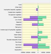
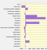
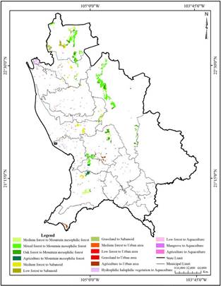
(Figure 3 ) describes gains and losses on land use categories at Nayarit during 1993-2014. Categories that have gained the largest areas in absolute values are agriculture (227,203 ha), mixed forest (194,222 ha), medium forest (166,616 ha); oak forest (151,089 ha), grassland (112,672 ha) and water bodies (12,183 ha). Oppositely, categories that have lost the largest areas in absolute values are: low forest (287,516 ha), oak forest (286,603 ha), medium forest (160, 927 ha), mixed forest (134,723 ha), grassland (116,909 ha) and agriculture (116,716 ha).
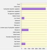
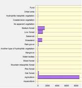
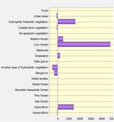
The expansion of aquaculture farms occurs at the expense of hydrophilic halophilic vegetation that lost 3,291 ha, mangroves lost 952 ha, agriculture lost 519 ha, and low forest which lost 364 ha (Figure 4). Agricultural expansion has affected low forests (47,711 ha), grasslands (33,066 ha), medium forest (27,559 ha), and oak forests (10,180 ha) (Figure 5). Urban expansion advanced over agriculture (8,727 ha), medium forests (1,513 ha), low forests (1,063 ha), grassland (964 ha) and oak forest (241 ha) (Figure 6).
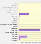
Mountain mesophilic forests seem to grow due to the contributions of mixed forests (29,456 ha), medium forests (13,888 ha), oak forests (11,680 ha), and agriculture (2,147 ha). (Figure 7). Water bodies growth is feed with the contributions of the low forest (4,808 ha), hydrophilic halophilic vegetation (1,623 ha), agriculture (1,478 ha), medium forests (520 ha) and the grasslands with 263 ha (Figure 8).
(Figure 9) is the map of change between land use categories in Nayarit for the period 1993-2014. It allows locating areas where change from one category to another occurred. Mesophilic forests have expanded over mixed forests, medium forests and oak forests, particularly in the upper and middle parts of the territory, as a process of forest area recovery. In contrast, sabanoid vegetation has gained territory due to contributions from the medium and low forests, grassland and oak forests, as a deterioration process of natural vegetation. Aquaculture farms expand over hydrophilic halophilic vegetation, mangroves, agriculture and low forests; these changes occur in the lower parts of the territory and closer to water bodies. Urban sprawl has removed agriculture, medium and low forests, grasslands and oak forests, as a result of the intense demand for new spaces for settlements.
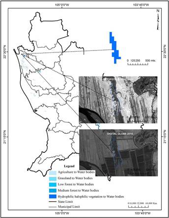
The map of contributions to net change in the category water bodies is shown in (Figure 10). Several areas of hydrophilic halophilic vegetation were transformed into water bodies. These changes are explained by the regional dynamism, given the demand of fresh water circulation for aquaculture farms. Artificial water bodies and new channels and channel connections are constantly built to provide water for the shrimp farms. In 1993, water bodies occupied 45,289.3 ha, which in 2014 increased to 53,092.00 ha, with a gain of 12,174.50 ha and a loss of 4,371.75 ha. Total change was of 16,546.25 ha, while the exchange was 7,802.75 ha. Finally, the net change was 8,743.50 ha.
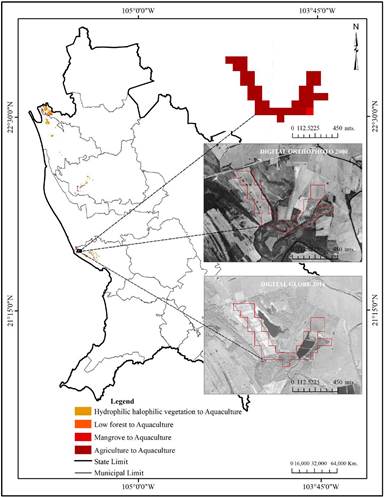
The contributions to the net change within the aquaculture farms are shown in (Figure 11). Agricultural areas were transformed into aquaculture farms; the image shows the construction of new shrimp farms and the expansion of their infrastructure. For 1993, the aquaculture farms occupied an area of 4,096.8 ha, while for 2014, it increased to 9,297.25 ha, obtained a gain of 5,291.51 ha and a loss of 91.00 ha. The total change was 5,382.50 ha, the exchange was 5,200.50 ha, and the net change was 182 ha.
Discussion
Studies of changes in land use and vegetation have been widely used to understand the dynamics of changes at the local and regional scale (Calderón-Loor et al., 2021; Calzada et al., 2018; Naikoo et al., 2020; Pérez-Hoyos et al., 2020). Change matrix indeed allow analyzing change processes into greater detail, especially regarding the contributions to net change and the exchanges occurring between categories (Camacho Sanabria, 2017; Pineda Jaimes & Santana Castañeda, 2019; Roldán-Aragón & Sevilla-Salcedo, 2014). It is remarkable the growth of aquaculture farms which expands over hydrophilic halophilic vegetation; such transformation is transcendental because it is permanent. Hydrophilic halophilic vegetation surface was reduced without recovery.
In general terms, there is a trend of expansion in the surface devoted to productive activities such as agriculture, aquaculture and urban spaces; while a considerable decrease occurs in areas with natural covers such as oak forests and low forest. In this sense, our results agree with those obtained by Berlanga-Robles & Ruiz-Luna (2020), Berlanga Robles et al., (2009) and Ramírez-Garcı́a et al. (1998), which show that agricultural and aquaculture farms have advanced over natural covers, being low forest and hydrophilic halophilic vegetation the most affected. Agricultural frontier expansion has an environmental impact and is expressed in the increase of grain sorghum, mango and sugar cane crops that have a greater representation of planted area according to the national agricultural survey (INEGI, 2014). Traditional crops such as: white corn and beans, occupy 30,571 ha in Rosamorada, 27,754 ha in Tepic and 22,712 ha in Compostela.
Agricultural fields also have been affected by urban sprawl, particularly in Tepic and Bahía de Banderas, due to the tourism and housing demand explained by the economic boom that Nayarit experienced from 1970 to 2015. Urban growth increased the pressure over natural resources in this region. Urban sprawl is also related to changes in land tenure regulations, the landowners and how they manage their lands determine the dynamics of the landscape. In Nayarit, aquaculture activity started in 1979 with a rustic system in the Estero El Conchal. In 1993 there were 4,096.8 ha devoted to aquaculture farms, which in 2014, increased to 9,297.25 ha, being hydrophilic halophilic vegetation (3,291 ha) and mangroves (952 ha) transformed into shrimp farms. Despite covering a small proportion of the landscape, such farms also represent a significant displacement of the hydrophilic halophilic vegetation. Mangroves lost is added as another factor of pressure on the surrounding natural wetlands, not only due to the possibilities of changing the land use and natural hydrological flow, but also through the contribution of nutrients and pollutants to water bodies and the spread of diseases (Páez-Osuna, 2001). Mangroves are located in low-lying coastal wetlands and are periodically submerged by incoming tides. Therefore, they are affected by the construction of roads, canals and ponds, which interfere with the surface flows of fresh and tidal water in the lagoon system (Blanco et al., 2011). The passage of Hurricane Rosa on October 14, 1994 caused a reduction in stem density and basal area in the mangroves of 31% and 51%, respectively (Kovacs et al., 2001). The loss of coverage caused directly by the meteor is estimated at approximately 600 has, and has been considered as a main disturbing event (Berlanga-Robles & Ruiz-Luna, 2007).
The use of information contained in attributes of the vegetation types map as one that provides the maximum level of detail of the analyzed geographic unit according to the work scale yielded a precision and accuracy of 95% for series II and the SNIEG digital quality information standard for series VI.
Conclusions
Detected changes in Nayarit during the study period are mainly associated with the expansion of agriculture and aquaculture farms as well as urban sprawl. Very dynamic change processes have been experienced in the State of Nayarit, fundamentally sustained by the growth of anthropic land uses (having an average growth of 4.62%) and forest shrink of 5.18%. According to the time-space dynamics of land use, 58.06% of the vegetation types and water bodies did not suffer any change while 41.94% showed some change in land cover, out of which 15.42% corresponds to exchanges between categories and 26.52% is a net change. Agriculture was the category that gained the most surface with an increase of 3.97%, while low forest lost the most surface (7.06%).
There are recovery and re-vegetation processes in the state, but do not have the same intensity than the disturbances, particularly in the low forest, oak forests and hydrophilic halophilic vegetation where recovery was low. Such processes are mostly driven by productive activities, due to the expansion of agricultural and aquaculture frontiers. The constant pressure of agricultural activities coupled with urban sprawl over forest resources, drive the dynamics of land use and water bodies changes, modifying the landscape and its biodiversity. Forest loss, particularly of the hydrophilic halophilic vegetation and mangroves is reflected in the contributions to the net change, which expresses the expansion of the aquaculture farms, which due to its high profitability have strongly increased.
Hopefully, this quantitative and qualitative vision of the conditions of natural resources and their spatio-temporal dynamics in Nayarit might help government agents to make better planning decisions, integrating socioeconomic development and environmental protection.

