


 English (pdf)
 Article in xml format
 Article references
 Send this article by e-mail
 Cited by SciELO
  Similars in
SciELO
Similars in
SciELO  uBio
uBio 
 Permalink
Introduction
Hydroelectric dams have several impacts on migratory fish, such as decreasing their abundance, local extinctions, and changes in assemblage structure (Agostinho, Miranda, Bini, Gomes, Thomaz & Suzuki, 1999; Agostinho, Thomaz, & Gomes, 2005; Franchi et al., 2014). In drainage basins, impacts reduce downstream floodplains and interrupt migratory fish movement (Dugan et al., 2010; Gandini, Sampaio, & Pompeu, 2014), impacting the availability of food resources (Zheng et al., 2018) and the reproductive success of species (Pompei, Lorenzoni, & Giannetto, 2016). In fact, the implementation and operation of large dams entirely change the physical characteristics of river floodplains (Ritcher, Baumgartner, Powell, & Braun, 1996), being more drastic downstream (Weber et al., 2013).
Environmental changes can select variations in life history attributes (Stearns, 2000; Reznick, Bryant, & Bashey, 2002), phenotypic plasticity occurs in several fish species (Reznick et al., 2002). Several studies on trophic morphology (e.g., Morita & Suzuki, 1999) and life history traits demonstrate variability in morphological traits (Mazzoni & Iglesias-Rios, 2002) and first maturation size class (Mérona, Mol, Vigouroux, & Chaves, 2009; Ferreira, & Godinho, 1990; Agostinho, Pelicice, & Gomes, 2008), exemplifying how ecological plasticity can explain the persistence of populations in impacted environments, such as dammed rivers (Pereira, Agostinho, & Delariva, 2016).
In lotic environments, food resources availability is defined by headwater-mouth longitudinal processes (Vannote, Minshall, Cummins, Sedell, & Cushing, 1980) and lateral input through the flooding pulse (Junk, Bayley, & Sparks, 1989). Therefore, damming changes longitudinal processes significantly by interrupting their continuity (Ward & Stanford, 1983, Ward & Stanford, 1995). Feeding pattern changes according to variations in a river’s hydrological cycle, especially when autochthonous (Roach, Winemiller, & Davis, 2014) and allochthonous production increases. Variations on autochthonous and allochthonous productivity are related to hydrological cycles since a lot of side material comes to the river during flooding in the rainy season (Junk et al., 1989). These cycles can alter resource availability (Rezende & Mazzoni, 2006; Rezende, Lobón-Cerviá, Caramaschi, & Mazzoni, 2013) and therefore, trophic niche breadth, which is an important parameter to the degree of trophic specialization (Amundsen, Gabler, & Staldvik, 1996). Niche breadth is expressed by relationship between composition and abundance of consumed items and high values can result from a population composed of generalist or specialist individuals (Bolnick, Yang, Fordyce, Davis, & Svanbäck, 2002). Species adaptation to environmental changes is associated with generalist habits and trophic plasticity (Krebs, 1989).
Flow regime acts as a selective factor for freshwater fish reproductive strategies (Mims & Olden, 2013). Reproductive strategies can be inferred through the analysis of life history traits that shows how variabilities are vital for populations (Stearns, 1976; Winemiller & Rose, 1992). Environmental characteristics can influence traits such as size at first maturation, clutch size, and parental care (Reznick et al., 2002; Tedesco et al., 2008).
Leporinus piau Fowler, 1941 is a migratory fish belonging to the family Anostomidae, the second in number of species of the order Characiformes (Ramirez, Birindelli, & Galleti-Jr, 2017). The anostomids are restricted to the Neotropics and are broadly distributed through South America; the genus Leporinus occurs in the cis and trans-Andean regions, from Trinidad Island to the North of Argentina (Garavello, Reis, & Strauss, 1992). Leporinus piau is a mid-sized species that reaches 25 cm in standard length and is broadly distributed in semiarid climate (Ramos, Ramos, & Ramos, 2014). Previous researchers have reported that, the migratory routes of this species can be impacted by dams (Araújo, Oliveira, Costa, & Novaes, 2016). Migration occurs in the main river basins of the region, including the São Francisco (Arantes et al., 2017) and Parnaíba river Basins (Ramos et al., 2014), as well as intermittent river basins that drain into the Atlantic Ocean. Although it is not the most abundant species in this region or threatened by anthropic pressures, it provides a relevant contribution to artisanal and sport fishing (Araújo et al., 2016). According to the assumptions of the life history theory, we hypothesize that the trophic and reproductive strategies of L. piau differ between sites located upstream and downstream from the Boa Esperança Dam, in the Parnaíba river. Based on this hypothesis, we tested the predictions: (1) diet composition will be more restricted and niche breadth will be smaller downstream from the dam, (2) the condition factor will be lower in the population downstream from the dam, and (3) size at first maturation will occur earlier in the downstream population.
Materials and methods
Study site: Parnaíba River drainage basin is around 330 000 km²; most of the main river is located in Piauí state. The air average temperature is 27 ºC, precipitation is around 1.726 mm/year and annual evaporation is around 1.517 mm/year (Ramos et al., 2014). Boa Esperança Dam is a hydroelectric power plant that started operating in April 1970 (Companhia Hidro Elétrica do São Francisco e Parnaíba, 2017); it is around 120 km long. We carried out sampling from August 2015 to July 2017 in the middle course of the Parnaíba river, in two lotic sites that were 220 km apart, Uruçuí (Sa) and Floriano (Sb).
Sampling: In each site, we set up three sampling stretches within a 2 km area to sample fish and record physicochemical parameters; the sampling stretches were located at opposite extremes ranging a distance of 1 km from the sampling stretch. Between August 2015 and July 2017, we collected specimens of L. piau two days per month, comprising a total of 48 sampling events at each site (Sampling permission # 51281-1 ICMBio). We used three methods to capture fish: gillnets, with 4, 5 and 7 cm between opposite knots; cast net, with 1 cm between opposite knots; and artisanal traps, made out of PET bottles.
Gillnet sets comprised three nets. Each net measured 20x1.5 m (30 m²) and was used twice at each site (180 m² in each point, 540 m² in each site). The gillnet sets soaked for 12 h, i.e., nets were deployed at sunset and removed at sunrise, totaling 24 h per week per site (96 h per point in each month; 288 h per site in each month; 3 456 h per year at each site). We checked nets every three hours or whenever necessary.
We used the cast net five times at each point, always in the morning between 08:00 and 10:00, with throws made at 10 min intervals at each site. Before throwing nets, we attracted fish with residues from leaves, cassava roots (Maniot esculenta Crantz), and crushed corn kernels (Zea mays spp.).
We used PET bottle traps as an additional sampling method during the rainy season, since water flow increased significantly, preventing fish sampling with gillnets or a cast net at site Sb. The traps were green and cut with scissors at the upper part of the bottle to form a funnel that hindered the exit of animals. The trap was placed on the bottom of the river by free diving, at 10 m from the margin, with a bait prepared with babassu coconut oil residue (Attalea speciosa Martius). The trap also contained gravel that was 5-7 cm in diameter, which fixed the trap on the bottom of the river, preventing it from being carried away by the flow. The trap entry was always facing downstream. After approximately 10 min, the trap was removed by free diving, and the diver closed the entry with one hand to prevent the animals from escaping. This procedure lasted approximately one hour, once a month, at the central point of the site. We calculated the catch-per-unit-effort (CPUE) for each trap with the formula CPUE = N / T -1 (adapted from Araújo et al., 2016) where N is the number of individuals captured and T is the time in hours.
After sampling, we anesthetizedthe L. piau specimens with clove oil (eugenol) at a concentration of 150 mg/L in an immersion bath, for later freezing. Then, we took the fish in thermal boxes to the Laboratory of Biodiversity and Bioarcheology of the UNIVASF Campus Serra da Capivara, in São Raimundo Nonato, state of Piauí. In the laboratory, fish were fixed in formalin (10 %) and, 24 h later, preserved in alcohol (70 %). Then we measured (cm) and weighed (g) all specimens and started dissection, which consisted of the removal of the digestive tract and gonads through an abdominal incision. These organs were preserved (alcohol 70 %) for later analyses. Voucher specimens of L. piau (CHNUFPI 27, 14 specimens; CHNUFPI 28, 17 specimens; CHNUFPI 29, 22 specimens) collected during the samplings were deposited in the Coleção de História Natural da Universidade Federal do Piauí in Floriano city, Brazil.
Environmental analyses: We recorded monthly abiotic variables with probes: Hanna HI 9146 (dissolved oxygen and water temperature) and Hanna HI 92000 (conductivity and pH). We obtained those parameters in the field making three measures at a depth of 2 m. We obtained river level, flow, and rainfall data from the São Francisco Hydroelectric Power Company website (CHESF, 2017). São Francisco Hydroelectric Power Company recorded these data at Ribeiro Gonçalves (7º34’01” S & 45º14’36” W) and Floriano-Barão de Grajaú (6º45’26” S & 43º01’57” W), approximately 70 km upstream from Uruçuí (Sa) and 30 km downstream from Floriano (Sb), respectively.
Laboratory analyses: We classified stomach repletion by visual observation according to volume content; following range: 0, 25, 50, 75, and 100 % of diet content in relation to maximum volume of the stomach. After that, stomach content was placed on a gridded petri dish and food items were identified using a stereomicroscope. We estimated the volume of each item in cubic centimeters, using a petri dish and mm-gridded paper (Hyslop, 1980; Albrecht & Caramaschi, 2003a, Albrecht & Caramaschi, 2003b). We used taxonomic keys, Merrit and Cummings (1996) and Mugnai, Nessimian, and Baptista (2010), to identify food items. Items offered as bait on sampling traps were not considered in the analysis. In total, we analyzed 530 stomachs of 260 individuals from the upstream population and 270 individuals from the downstream population. Among the stomachs analyzed, 41 upstream and 57 downstream samples showed no repletion degree.
Gonads of the individuals collected were classified into (1) immature, (2) at precocious maturation, (3) mature, (4) spent, through the observation of macroscopic aspects (Vazzoler, 1981; Brown-Peterson, Wyanski, Saborido-Rey, Macewicz, & Lowerre-Barbieri, 2011). The condition factor was calculated for each individual through the formula: K = Wt Lsb, where Wt = total weight, Ls = standard length, and b = angular coefficient (Le Cren, 1951). We calculated the gonadosomatic index (GSI) for each individual with the formula GSI = Wg Wt × 100, where Wg = gonad weight and Wt = total weight.
Statistical analyses: We applied a principal component analysis (PCA) to a correlation matrix to test for possible site groupings, but before that, the variables were submitted to a collinearity analysis
We applied the a priori Shapiro-Wilk test to all data to test normality and homoscedasticity. Permutational multivariate analysis of variance (PERMANOVA) (Anderson, 2017) and SIMPER analyses (Clarke, & Warwick, 2001) were applied to the diet data matrix, which contained the volume of each item, in order to test differences in diet between sites. We also checked niche breadth by using the test of homogeneity of multivariate dispersions (PERMDISP) (Anderson, 2006).
We applied the PERMDISP test to diet data assuming that trophic niche difference was expressed by distance from each individual to the multivariate average of its group (Anderson, 2006; Correa & Winemiller, 2014). The test was applied to the matrix of diet similarity composed of volumetric data, and the analysis was generated using the R software, in the Vegan Package (Oksanen et al., 2019). We used residual permutation (999 permutations) to calculate probability values (Anderson, 2006).
We calculated the length-weight relationship plotting the total weight (Wt, [g]) on the standard length (Ls [cm]) for each site with a linear regression, using log-transformed data and the following log10 formula: Wt = a + b log10 Ls, where “a” and “b” are regression constants (Froese, 2006). We also tested the b-value difference with Student t test. Additionally, we tested curves generated for each site data using ANCOVA (Analysis of covariance); weight and size were used as the dependent variables, site as the independent variable, and standard length as the covariable. We estimated the size at first maturation (L 50) to evaluate the results of the gonad observations. This estimation occurred through the proportional verification of the average length in which 50 % of the individuals were at the 2, 3 and 4 (mature) maturation stages. We tested these values using the ANCOVA test, through Generalized Linear Models (GLM) generated from site and sex data, with confidence intervals with 999 iterations (Bootstrap).
Two Linear Mixed Models (LMM) were performed to test the influence of season, sex, and site on the condition factor (K) and the gonadosomatic index (I G). For each response variable, the condition factor (K) and the gonadosomatic index (I G) were tested with three models, including all possible combinations of the explanatory variables. In the models, season and sex were selected as fixed effect variables and site as the random effect variable. The model with the lowest value for Akaike’s Information Criterion (AIC) was considered the best fit, and then, the others were ranked according to the differences calculated between AICs (ΔAIC). In order to determine the relative significance of the models, the Normalized Akaike’s Weight (W im ), where W im = exp (-0.5 × ΔAICi) ∑R, r = 1 exp (-0.5 × ΔAICi)-1 was calculated (Johnson, & Omland, 2004). ANOVA was used to test the significance of the best-fitted model. In addition, Wald Chi-square Tests were performed to verify the significance in model interactions variables.
Statistical analyses were performed using packages ade4 (Dray, & Dufour, 2007), car (Fox, & Weisberg, 2011), FSA (Ogle, 2018), lme4 (Bates, Maechler, Bolker, & Walker, 2015),nlstools (Baty et al., 2015), USDM (Naimi, Hamm, Groen, Skidmore, & Toxopeus, 2014), and vegan (Oksanen et al., 2019) in R Software (R-Team, 2016).
Results
Environmental characterization: PCA identified two groups (downstream and upstream) according to environmental variables: water temperature, conductivity, river level, flow, and rainfall (Fig. 1).
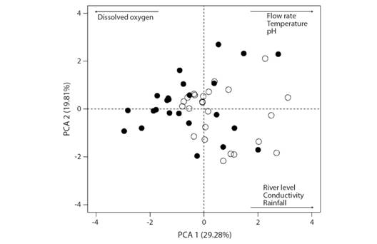
Fig. 1 Principal component analysis (PCA) of the environmental data from middle Parnaíba River, Piauí State, Brazil. Black and white circles represent the upstream and downstream sites, respectively.
Fish sampling: We collected a total of 801 L. piau specimens; 391 upstream and 410 downstream. The most efficient method of capture was the PET bottle trap, with CPUE = 6.83 ind./h. The cast net was the second most efficient method, with CPUE = 0.6 at the upstream site and 0.31 ind./h at the downstream site. The gillnets showed the lowest CPUE; 0.007 upstream and 0.005 ind./h downstream. Upstream, we collected 272 individuals in the dry seasons and 119 in the rainy seasons, whereas downstream, we collected 214 individuals in the dry seasons and 196 in the rainy seasons. The cast net captured 232 specimens upstream and 122 downstream, followed by gillnets, with 159 specimens upstream and 124 downstream. The PET bottle trap collected a total of 164 individuals.
Trophic ecology: Diet was composed of 29 food items from all samples, including upstream and downstream sites (Table 1). PERMANOVA results recorded significant differences between sites (pseudoF = 4.16, P < 0.01). SIMPER analysis showed that difference between sites was determined by the items unidentified organic matter (average dissimilarity = 0.21, standard deviation = 0.25, ratio = 0.81, cumulative contribution = 0.57, P= 0.01) and plant fragment (average dissimilarity = 0.86, standard deviation = 0.17, ratio = 0.49, cumulative contribution = 0.77, P= 0.03). PERMDISP showed that upstream and downstream trophic niche breadth were significantly different (F = 8.23, P= 0.004) (Fig. 2).
TABLE 1 Relative frequency (%Fi) and relative volume (%V) of food items of Leporinus piau recorded upstream and downstream of Boa Esperança Dam, Parnaíba River, Piauí State, Brazil
| Upstream | Downstream | ||||
| Fi (%) | V (%) | Fi (%) | V (%) | ||
| Chlorophyta | |||||
| Green algae | 5.38 | 2.84 | 8.82 | 1.32 | |
| Lignophyta | |||||
| Poacea seeds | 24.73 | 45.97 | 26.47 | 93.77 | |
| Fruit remains | 1.43 | 1.12 | 0.98 | 0.05 | |
| Vegetal fragments | 14.34 | 11.38 | 8.5 | 0.57 | |
| Leaves | 0.72 | 0.83 | 0.98 | 0.01 | |
| Hydrocharytaceae | 0.33 | 0.08 | |||
| Nemathelminthes | |||||
| Nematodea | 0.36 | 0.07 | 1.31 | 0.09 | |
| Arthropoda | |||||
| Arachnida | 0.36 | 0.02 | |||
| Insecta | |||||
| Insect fragments | 0.72 | 0.07 | 3.27 | 0.05 | |
| Insect larvae | 0.36 | 0.2 | 1.31 | 0.02 | |
| Diptera (Stratiomyidae) | 0.65 | 0.03 | |||
| Diptera (Simulidae) | 0.33 | 0.01 | |||
| Ephemeroptera 1 | 3.27 | 0.23 | |||
| Ephemeroptera (Baetidae) | 0.65 | 0.05 | |||
| Coleoptera | 1.08 | 0.04 | 0.98 | 0.03 | |
| Trichoptera | 0.36 | 0.1 | 1.63 | 0.06 | |
| Hymenoptera | 0.72 | 2.65 | 1.31 | 0.02 | |
| Plecoptera | 0.33 | 0.01 | |||
| Lepdoptera | 0.65 | 0.06 | |||
| Amphipoda | 0.33 | 0.03 | |||
| Isopoda | 0.36 | 0.01 | 0.65 | 0.02 | |
| Crustacea | 0.72 | 0.11 | 1.96 | 0.08 | |
| Decapoda | 1.31 | 0.47 | |||
| Chordata | |||||
| Actinopterygii | |||||
| Scales | 6.45 | 0.43 | 4.58 | 0.1 | |
| Fish bones | 1.79 | 0.39 | 0.98 | 0.19 | |
| Characiformes | 0.72 | 0.88 | |||
| Muscle | 10.75 | 6.85 | 11.11 | 1.05 | |
| Others | |||||
| Unidentified organic matter | 27.6 | 25.69 | 15.69 | 1.59 | |
| Sediment | 1.08 | 0.36 | 1.63 | 0.03 | |
| Total items | 20 | 27 | |||
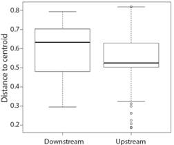
Fig. 2 Trophic niche breadth variation of Leporinus piau in sites upstream and downstream from the Boa Esperança Dam, Parnaíba River, Piauí State, Brazil.
Life history: The weight-length relationship was described for log10 Wt = - 4.8291 + 3.0795 Log10 Ls (r2 = 0.9778) upstream and log10 Wt = -4.621 + 2.9718 Log10 Ls (r2 = 0.9731) downstream site. Upstream minimum, maximum, and median lengths were 5.70 cm, 30.69 cm, 13.02 cm, respectively and the standard deviation was 3.58. Downstream minimum, maximum, and median lengths were 5.76 cm, 23.97 cm and 11.80 cm, respectively and the standard deviation was 2.72. The b-value in the regression for the population upstream was significantly different from 3 (t = 3.37, P= 0.0008), whereas the b-value in the regression for the population downstream was not significantly different from 3 (t = -1.15, P= 0.249). The curves differed significantly between populations (F = 9.96, P= 0.001)
The estimated lengths at first maturation were L 50 = 10.74 cm and L 50 = 10.57 cm for females and L 50 = 12.64 cm and L 50 = 10.92 cm for males, upstream and downstream respectively. There were significant differences in L 50 between sites for female (z = 6.39, P< 0.05) and males (z = 5.94, P< 0.05).
The best fitted LMM model for the Conditional Factor (K) had as fixed effect variable season and sex, and site as the random effect ((K~ Sex+(1|Site)) (Table 2). Demonstrating that variation in K was not explained by site. The intercept of ex (random effect) showed zero as variance and standard variation, which demonstrates that sex varies across seasons. This result was corroborated by the Wald Chi-square test in which K was significantly different between seasons (χ2 = 10.70, d.f. = 1, P< 0.05) (Fig. 3).
TABLE 2 Results of the Linear Mixed Model (LMM) analysis for the response variables, condition factor (K) and gonadosomatic index (I G), and predictive variables, season, sex, and flow, gathered at sites upstream and downstream from the Boa Esperança Dam, Parnaíba River, Piauí State, Brazil (AIC = Akaike’s Information Criterion; W im = Akaike’s weight)
| Model (LMM) | AIC | ΔAIC | W im |
| Condction Factor | |||
| • Sex+(1|Site) | -598.43 | 0 | 0.43 |
| • Season+Sex+(1|Site) | -597.16 | 1.27 | 0.23 |
| • Sex+Flow+(1|Site) | -596.62 | 1.81 | 0.17 |
| • Season + Sex+Flow+(1|Site) | -595.39 | 3.04 | 0.09 |
| • Season +(1|Site) | -592.88 | 5.55 | 0.02 |
| • Flow+(1|Site) | -592.33 | 6.10 | 0.02 |
| • Season +Flow(1|Site) | -591.06 | 7.37 | 0.01 |
| GSI | |||
| • Season +Sex(1|Site) | -262.49 | 0 | 0.49 |
| • Season +Sex+Flow+(1|Site) | -262.14 | 0.35 | 0.41 |
| • Sex+Flow+(1|Site) | -258.86 | 3.63 | 0.08 |
| • Sex+(1|Site) | -248.09 | 14.40 | 0.0003 |
| • Season +(1|Site) | -238.35 | 24.14 | 3-6 |
| • Season +Flow+(1|Site) | -237.44 | 25.05 | 1.88-6 |
| • Flow(1|Site) | -236.30 | 26.19 | 1.07-6 |
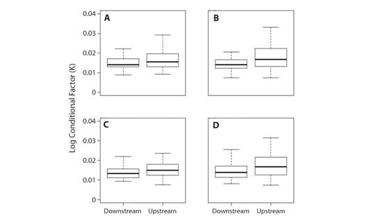
Fig. 3 Condition factor logarithm (K) between seasons and sexes at sites upstream and downstream from the Boa Esperança Dam, Parnaíba River, Piauí State, Brazil. a) Female Rainy Season, b) Female Dry Season, c) Male Rainy Season and d) Male Dry Season.
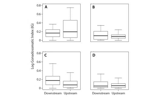
The best fitted LMM model for Gonadosomatic Index (I G) had site as the fixed effect variable, and sex as the random effect variable (I G ~ Site (1|Sex)) (Table 2). The intercept variance of sex (random effect) was 0.02 and with a standard variation of 0.13, showing that I G of females and males indicate differences between sites. The Wald Chi-square test corroborated this result (χ2 = 12.05, d.f. = 1, P< 0.05) (Fig. 4).
Discussion
Environmental variables (flow, temperature, pH, river level, conductivity, and rainfall) grouped the two sites. According to Willis, Winemiller and Lopez-Fernandez (2005), flow is a structuring factor of fish assemblages owing to material loading from marginal areas that makes the environment more heterogeneous. Jepsen, Winemiller and Taphorn (1997), studying cichlids in Venezuela, showed that resources are partitioned among species of the genus Cichla as a function of hydrological fluctuation, which affects the use of habitat for feeding and reproduction. There is high variation in habitat use in the genus Leporinus (Araya, Agostinho, & Bechara, 2005); species can use the main channel bottom of large rivers, lagoons, and small streams, where physicochemical parameters, especially dissolved oxygen, have less variation, (Weber et al., 2013). L. piau likely selected the main channel bottom of the Parnaíba river owing to less variation in the abiotic factors.
L. piau showed a predominantly omnivorous diet at both sites, mainly composed of plants, but were determined to have significant differences between them based on the variation in the abundance of some food items. Niche breadth was more variable downstream where L. piau also consumed a larger number of animal items. Species of the genus Leporinus showed changes in the diet with a greater tendency towards carnivory in rivers impacted by dams (Albrecht, & Caramaschi 2003a, Albrecht, &Caramaschi 2003b; Mendonça, Hahn, & Loureiro-Crippa, 2004). This is a common behavior since dams increase the abundance of alien species, negatively affecting the condition of native species (Giannetto et al., 2012), causing sensitive species to spread and occupy areas less affected by the presence of competitors (Pompei, Lorenzoni, & Giannetto, 2016; Pompei, Giannetto, & Lorenzoni, 2018). The increase in niche breadth and the higher richness of items in the downstream site showed that the diet of L. piau was altered by environmental changes in the Parnaíba river.
The life history theory predicts that an increase in the size of individuals benefits the species owing to a higher production of offspring (Stearns, 1992, Stearns, 2000). We observed that the investment in somatic growth was higher, and size at first maturation occurred later at the upstream site than at the downstream site. In populations of the same species, life history attributes can vary owing to variations in conspecific densities or environmental variations (Stearns, 1992, Stearns, 2000; Reznick et al., 2002). At the downstream site, earlier onset of maturation may result from high density, predation, or decrease in resources and consequently, will cause a decrease in the theoretical maximum size (Reznick et al., 2002). The onset of maturation and the reduction of the theoretical maximum size downstream can result from the quality of the resource consumed, at this site, algae was fond in higher concentrations in the diet. Algae are resources with low energetic quality, and their consumption can decrease growth in the population (Bowen, Lutz, & Ahlgreen, 1995) as we observed in L. piau in the Parnaíba river.
The results of the LMM showed that the best fitted model for the condition factor showed “sex” as the fixed parameter and “site” the as random parameter. At the downstream site, both sexes showed significantly higher condition factor values, which can be related to the consumption of food items of high nutritional quality, such as invertebrates (Bowen et al., 1995). High condition factor values can also be related to the food availability and use by individuals (Fulton, 1902). In the case of L. piau, this difference can be related to nutrition conditions (Bowen et al., 1995), as at the downstream site, items of animal origin (invertebrates) were more abundant in their diet.
In the best fitted GSI model, the fixed parameters of the LMM were “season” and “sex,” in which the highest value corresponded to the females in rainy seasons when the water flow (flow) was higher. Usually, Anostomidae species have higher GSI values during the rainy season since females have greater total weights due to mature ovaries (Villares Junior, Gomiero, & Goiten, 2011; Araújo et al., 2016). In this sense, Anostomidae reproduction is related to rainy season and environmental factors such as high water temperatures and photoperiod that are considered triggers for maturation and spawning (Thomé, Bazzoli, Rizzo, Santos, & Ratton, 2005).
In conclusion, diet composition differed between sites, niche breadth and item richness were both higher downstream. These results did not support our first prediction. In the downstream site, conditional factor was lower and size at first maturation occurred earlier corroborating our second and third predictions. These results suggest that the life-history traits of L. piau differ between the two sites. In the upstream site, weight-length ratios had a higher slope (b = 3.08) than downstream, demonstrating faster growth. Reproduction was delayed since size at maturation was higher upstream. Reproductive effort (GSI) had smaller values and higher variation, suggesting a population strategy of growth investment and delayed reproduction. Those characteristics were related to a more stable environmental (Stearns, 1992). According to life history theory, environmental variations can lead to phenotypic plasticity of life-history traits related to reactions norms (Stearns, 2000). This process that can occur in fishes from dammed rivers (Mérona et al., 2009) as a short-term adaptation (Stearns, 1992). Life-history traits recorded at the upstream site were similar to those of lentic habitats, resulting in larger individuals, reproduction delay, and less reproductive effort. Environmental variables (water temperature, photoperiod, season, and flow), conspecific densities, predation and competition can affect organisms’ reproductive traits (Stearns, 1992, Stearns, 2000; Reznick et al., 2002). Therefore, it is not possible to identify the selection agent in the field. However, these results exemplify the variability predicted by life history theory, as an explanation of the dam’s impact on the life history of L. piau.
Ethical statement: authors declare that they all agree with this publication and made significant contributions; that there is no conflict of interest of any kind; and that we followed all pertinent ethical and legal procedures and requirements. All financial sources are fully and clearly stated in the acknowledgements section. A signed document has been filed in the journal archives.

