


 English (pdf)
 Article in xml format
 Article references
 Send this article by e-mail
 Cited by SciELO
  Similars in
SciELO
Similars in
SciELO  uBio
uBio 
 Permalink
Release of aquaculture stocks (purposely or inadvertently) may modify the genetic composition and variability of wild populations, resulting in issues that may compromise long term fitness (Utter, 2003). Potential genetic risks are an increase in the rate of inbreeding, homogenization of the genetic structure, displacement of genes adapted to local conditions, and modification of adaptability by domestication (FAO, 1993; Hallerman, Brown, & Epifanio, 2003; Miller & Kapuscinsky, 2003; Taniguchi, 2004; Habtemariam, Arias, García-Vázquez, & Borrell, 2015; Bylemans et al., 2016).
The genetic makeup of cultivated stocks is usually different from their wild counterparts, including reduced genetic variation; this has been documented for several seafood species, including red sea bream Pagrus major (Perez-Enriquez, Takagi, & Taniguchi, 1999), flatfishes, e.g. Hippoglossus hippoglossus and Scophthalmus maximus, (Danancher & Garcia-Vazquez, 2011), cod Gadus morhua (Glover, Dahle, & Jørstad, 2011), grooved carpet shell clam Ruditapes decussatus (Borrell et al., 2014), and Australian blacklip Haliotis rubra and South African H. midae abalones (Evans, Bartlett, Sweijd, Cook, & Elliott, 2004). For the Pacific whiteleg shrimp Litopenaeus vannamei (Boone, 1931) and other farmed shrimp species, such as the kuruma and giant tiger prawns, this reduced genetic variation has also been reported (Freitas & Galetti, 2005; Perez-Enriquez, Hernández-Martínez, & Cruz, 2009; Mendoza-Cano, Grijalva-Chon, Perez-Enriquez, Ramos-Paredes, & Varela-Romero, 2013; Vela-Avitúa, Montaldo, Márquez-Valdelamar, Campos-Montes, & Castillo-Juárez, 2013; Knibb et al., 2014). Inbreeding depression that affects shrimp performance traits, including survival and susceptibility to viral infection, has also been documented (Bierne et al., 2000; Keys et al., 2004; De Donato, Manrique, Ramírez, Mayer, & Howell, 2005; Moss, Arce, Otoshi, Doyle, & Moss 2007; Goyard et al., 2008).
Examples of the impact of farmed species on the genetic structure of wild populations come from studies in fish and mollusks. A risk assessment of Atlantic salmon indicates that many locations in Norway are at moderate or high risk of genetic introgression from farmed salmon (Taranger et al., 2015). Examples of low introgression from marine farming have also been documented for the European seabass Dicentrarchus labrax (Brown, Miltiadou, & Tsigenopoulos, 2015) and the great scallop Pecten maximus (Morvezen et al., 2016). Genetic impact of farming comes from introduced exotic shrimp: L. vannamei in Thailand (Senanan et al., 2007) and the giant tiger prawn in Colombia (Aguirre-Pabón, Orozco-Berdugo, & Narváez-Barandica, 2015), interact with the native counterparts. Assessments of the genetic impact of farming on the structure of native populations are still scarce. For the giant tiger prawn Penaeus monodon, Tassanakajon, Pongsomboon, Jarayabhand, Klinbunga, and Boonsaeng (1998) and Xu et al. (2001) found no conclusive evidence of an impact of farmed shrimp on wild populations, but suggested that more data has to be obtained.
In Mexico, L. vannamei is the most important aquaculture species, and the mean annual production in 2004-2013 was 102 000 Mt (CONAPESCA, 2013). The State of Sinaloa produces more than 50 % of national production. In 2015, the number of postlarvae sold by 34 hatcheries that operated in Mexico was about 10.5 billion (ANPLAC, 2016). Inadvertent release of large numbers of shrimp to the wild occurs on farms with earthen ponds during harvesting, hurricanes, or from hatcheries during larvae production. However, no estimates of the number of escapees are available. Thus, the hypothesis of this study was that, due to the large aquaculture activities taking place in the State of Sinaloa, possible signs of gene introgression of farmed shrimp into the wild would be detectable. For that purpose, the temporal genetic make-up of wild white leg shrimp living along the coast of the State of Sinaloa was compared with the genetic profiles of hatchery-reared stocks.
Materials and methods
Sampling: Samples of wild (2002, 2012, and 2013) and farmed shrimp were obtained. A total of 32 wild shrimps were collected at or near the mouth of each estuary, with 1-inch mesh throw nets, from three sites of the State of Sinaloa, Mexico: Yameto in 2002 (see Valles-Jiménez, Cruz, & Perez-Enriquez, 2005), Bahía del Colorado in November 2012, and Teacapán in September 2013 (Figure 1A). The collection point at Yameto (Wild-2002) is at the estuary Bahía de Santa María (24°47ʹ57ʺ N-108°03ʹ17ʺW), 7-9 km apart of the farming area (Figure 1B). The Bahía del Colorado point (Wild-2012; 25°40ʹ47ʺN-109°22ʹ40ʺW) at the Lechuguilla estuary, is located 12-13 km apart from the farming area (Figure 1C). At the estuary of Teacapán (Wild-2013; 22°32’37” N-105°45’42” W) the nearest shrimp farm is 5 km away from the collection site (Figure 1D).
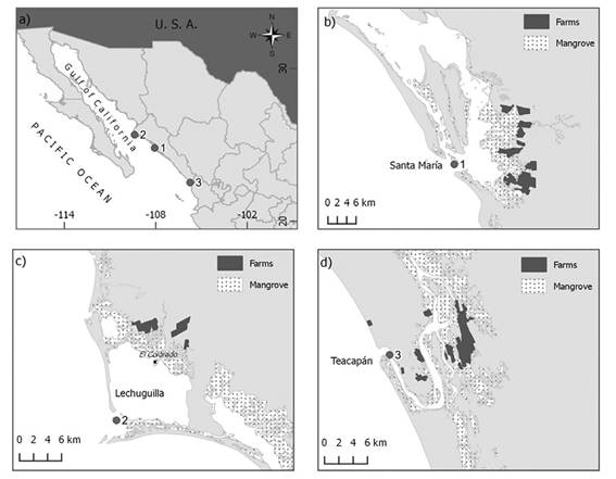
Figure 1 A) Sampling sites of wild shrimp Litopenaeus vannamei in the State of Sinaloa, Mexico. 1: Yameto (Wild-2002); 2: Bahía del Colorado (Wild-2012); 3: Teacapán (Wild-2013). B) to D) represent a detailed view of each collection site.
Farmed shrimps came from two commercial hatcheries sampled in 2007 (n = 32 each) located in the states of Sinaloa and Sonora, but both selling part of its larvae production within the State. From the data of Perez-Enriquez et al. (2009), these two hatcheries (named F and D) when pooled (data not shown), represented the genetic profile of six hatchery-reared stocks for Mexico in the year 2007. Pleopod tissue from each shrimp was preserved in 80 % ethanol, until DNA extraction was performed with the DNeasy Blood and Tissue Kit (Qiagen, Hilden, Germany).
Genetic analysis: The genetic characterization of shrimp consisted in obtaining microsatellite genotypes, for which a new set of microsatellite markers was developed. The marker panel development followed a pyrosequencing strategy in a Roche 454 platform (analysis by Macrogen, Seoul, South Korea). The FASTA sequences were analyzed by a PERL code (A. Munguía-Vega, personal communication) to eliminate sequences that presented ambiguities (“Ns” present), did not contain adapters at 5′, and were duplicated. Microsatellites were searched on the remaining sequences, using the software QDD (Meglécz et al., 2010), which implements CLUSTALW2 (Larkin et al., 2007), BLAST (ftp://ftp.ncbi. nih.gov/blast/executables/), and PRIMER3 (Rozen & Skaletsky, 2000) in a Perl5 platform (http://www.active state.com/activeperl/). A set of 80 pairs of primers was designed for perfect di-, tri-, and tetra-nucleotides with at least seven repetitions. The primers were designed with an optimum length of 20 nucleotides (range 17-25) and a melting temperature (Tm) of 60 °C (range 58-62), with a maximum difference of 2 °C between forward and reverse.
Fourteen of the 80 microsatellites showed adequate amplifications, which were chosen to characterize the sample from Bahía del Colorado. PCR reactions were done in 12 µL containing 20 ng of genomic DNA, 1× PCR buffer, 1.5 mM MgCl2, 0.2 mM each dNTP, 0.3 µM each primer (forward and reverse), and 0.025 U/µL Taq DNA polymerase (Promega). All primer pairs were run in a C1000 thermal cycler, with an initial denaturation at 94 °C for 3 min, 30 cycles of denaturation at 94 °C for 35 sec, annealing at 57 °C for 40 sec, and extension at 72 °C for 40 sec, and a final extension at 72 °C for 2.5 min. Microsatellite loci were genotyped by a genetic analyzer (ABI-3130, Applied Biosystems, Foster City, CA) with forward primers tagged with fluorescence with 6-FAM, VIC, NED, or PET. Alleles were read by GeneMapper 4.0 software (Applied Biosystems) and sizes classified in bins.
Number of alleles per locus (na), effective number of alleles (ne), observed (Ho) and expected heterozygosity (He), and deviation from Hardy-Weinberg equilibrium (HWE) were calculated for each microsatellite locus using Arlequin 3.5.1.3 program (Excoffier, Laval, & Schneider, 2005); the significance of HWE for each locus was corrected by the Bonferroni sequential method (Rice, 1989). The possibility of null alleles in loci deviating from HWE was assessed with the Microchecker software (Van Oosterhout, Hutchinson, Wills, & Shipley, 2004).
Allele frequencies of selected microsatellite loci were calculated to characterize wild and hatchery-reared shrimp. Temporal genetic diversity among wild samples and between pooled wild and hatchery-reared samples was compared by Student-t tests. Population differentiation was determined by global Fst and pairwise Fst by Arlequin 3.5.1.3 (Excoffier et al., 2005). Population structure was also inferred by a model-based clustering method implemented by STRUCTURE 2.3 software (Pritchard, Stephens, & Donnelly, 2000). The model assumes the presence of K populations, each characterized by a set of allele frequencies at each locus. Individuals in the sample are assigned probabilistically to populations. The running conditions for the Markov chain were 1 000 000 chain steps and 100 000 simulations for K = 1 through 5. The best K number of populations was calculated by the Evanno method (Evanno, Regnaut, & Goudet, 2005) implemented in the STRUCTURE HARVESTER software (Earl & von Holdt, 2012). A Principal Coordinates Analysis (PCoA) was used in GenAlEx 6.5 software (Peakall & Smouse, 2006, 2012) to visualize genotypic distributions, per individual and sampling site, in two dimensions. Assignment tests were done in Arlequin, GenAlEx and STRUCTURE programs to determine, based on the multilocus genotype, the most probable origin (wild or cultivated) of each individual collected in the wild. The number of shrimp from the wild samples that showed a genetic composition assigned to cultivated stocks was used to calculate the percentage of individuals of hatchery origin in the wild.
Results
The genetic diversity of the panel of fourteen microsatellites was in general high, with most loci varying between 9 and 16 number of alleles per locus, and expected heterozygosity values higher than 0.75 (Table 1). Five loci deviated from HWE (Table 1). Eleven loci were selected for the genetic characterization of wild and hatchery-reared samples based on genotypes reading quality. Average genetic diversity (na, ne, and He) was higher in the three wild samples than in the two hatchery-reared samples (Table 2); when samples were pooled into two groups (wild and hatchery-reared), the difference was statistically significant (P < 0.05). There were no significant differences in genetic diversity among wild samples, and a higher number of loci deviated from HWE in wild than in hatchery-reared samples (Table 2). According to the analysis with Microchecker deviations from HWE at several loci, that was consistent in all populations in loci Livan13 and Livan60, are explained by the presence of null alleles and/or stutters. These two loci were not used in the further analyses. In wild samples, deviations in Livan30 were not explained by null alleles.
Table 1: Genetic characterization of 14 microsatellite loci (repeat motif in parenthesis) in a sample of wild Litopenaeus vannamei from Sinaloa, Mexico
| Locus | Forward and reverse primer sequences (5′-3′) | Allele range | N | n a | Ho | He | HWE |
|---|---|---|---|---|---|---|---|
| Livan04a (ATTT)9 | ATTCTTGGAGTATGCGGTGG TGATTTGAGAACGAGACGGA | 134-174 | 28 | 12 | 0.750 | 0.860 | 0.240 |
| Livan09a (ACA)15 | AAAGTGACTGCCTGGCAACT TTTGAGGGCATGGAAACAGT | 172-203 | 20 | 13 | 0.600 | 0.835 | 0.024 |
| Livan10a (GGA)13 | ACAATGTAAACAAACCGGGC CGGTAGGATGAGGTTCCTGT | 172-194 | 29 | 13 | 0.759 | 0.858 | 0.107 |
| Livan12a (CAA)10 | AACCAACTCGGGATGACG GTGGGGGTGATCTTTTCCA | 115-133 | 23 | 8 | 0.783 | 0.848 | 0.055 |
| Livan13a (GTT)10 | AAAGTGCGGATATTAGTGTTTTTG TCTGCACGTCCTTCCTTTCT | 274-341 | 24 | 16 | 0.500 | 0.789 | 0.250 |
| Livan15 (ATT)10 | GCCAAATGGAGCCTAAGAAG TTTAATTTCGTCCGTCTGGC | 182-227 | 28 | 20 | 0.643 | 0.926 | <0.001* |
| Livan24a (ATT)7 | TCTTGTCGATGATGGTGATGA GCCCTTTGTGGCTTGTCTAA | 141-165 | 23 | 7 | 0.565 | 0.764 | 0.065 |
| Livan25 (TGG)7 | ACACAGGAGGTAATGGAGGC TGTATGGAGAGGAACCCCTG | 170-178 | 20 | 5 | 0.700 | 0.676 | 0.582 |
| Livan30a (TCC)7 | CCCATCTCTTTCGGTGGTTA GAACAGCGGAGGAGGAGAAT | 128-158 | 32 | 7 | 0.500 | 0.608 | 0.003* |
| Livan42a (CT)9 | TGTATGTATGCGTGCGTGTG CACTTCGCCATTTAATCCGT | 214-242 | 25 | 8 | 0.400 | 0.786 | 0.001* |
| Livan44a (TC)8 | ACCCTCTCATCAAGCAGTGG TCCACAGAAGAGCGTGTTTG | 232-256 | 28 | 13 | 0.571 | 0.883 | <0.001* |
| Livan51a (AG)8 | CAATTACTCCGGCCTCAAGA AACCGTACACAGGCCAATTC | 149-181 | 31 | 12 | 0.839 | 0.870 | 0.840 |
| Livan56 (TG)7 | TGTTGTGTCTCTTCGTTGCC TTTCGTAAAAGCTGTCGCAA | 125-149 | 20 | 16 | 0.500 | 0.879 | 0.004* |
| Livan60a (AT)10 | TGGCCGTAGATACTGACCCT CATGCAGGCTTGAAGAGTGA | 266-330 | 28 | 15 | 0.643 | 0.896 | 0.103 |
N = sample size, na = number of alleles, Ho = observed heterozygosity, He = expected heterozygosity, HWE = probability of deviation from Hardy-Weinberg equilibrium.
a Locus used for the genetic characterization wild samples.
* Significant after Bonferroni correction.
Table 2: Genetic diversity of wild and hatchery-reared samples at 11 loci
| Population | Livan04 | Livan09 | Livan10 | Livan12 | Livan13 | Livan24 | Livan30 | Livan42 | Livan44 | Livan51 | Livan60 | Mean | ||||
|---|---|---|---|---|---|---|---|---|---|---|---|---|---|---|---|---|
| Wild-2002 | ||||||||||||||||
| N | 30 | 17 | 29 | 32 | 13 | 30 | 31 | 21 | 29 | 29 | 24 | 25.9 | ||||
| na | 13 | 14 | 8 | 8 | 9 | 14 | 6 | 9 | 7 | 12 | 17 | 10.6 | ||||
| ne | 5.6 | 8.6 | 4.1 | 5.3 | 5.9 | 3.7 | 3.0 | 5.5 | 3.9 | 7.3 | 10.6 | 5.8 | ||||
| Ho | 0.767 | 0.824 | 0.724 | 0.813 | 0.308 | 0.600 | 0.516 | 0.429 | 0.552 | 0.621 | 0.500 | 0.605 | ||||
| He | 0.834 | 0.911 | 0.768 | 0.825 | 0.865 | 0.740 | 0.676 | 0.837 | 0.759 | 0.878 | 0.925 | 0.820 | ||||
| HWE | 0.515 | 0.501 | 0.882 | 0.725 | 0.002*,a | 0.006* | <0.001* | 0.068 a | 0.010n.s.,a,b | 0.032n.s.,a | 0.001*,a | |||||
| Wild-2012 | ||||||||||||||||
| N | 22 | 14 | 23 | 25 | 17 | 17 | 27 | 13 | 17 | 26 | 13 | 19.5 | ||||
| na | 11 | 9 | 9 | 9 | 10 | 11 | 6 | 8 | 9 | 12 | 11 | 9.5 | ||||
| ne | 4.3 | 7.0 | 5.0 | 7.2 | 6.9 | 7.2 | 3.2 | 5.0 | 4.3 | 6.5 | 7.7 | 5.8 | ||||
| Ho | 0.682 | 0.571 | 0.652 | 0.640 | 0.176 | 0.647 | 0.667 | 0.385 | 0.529 | 0.423 | 0.385 | 0.523 | ||||
| He | 0.784 | 0.889 | 0.816 | 0.878 | 0.881 | 0.888 | 0.703 | 0.831 | 0.793 | 0.863 | 0.905 | 0.839 | ||||
| HWE | 0.007* | 0.015 n.s.,a | 0.548 | 0.036n.s.,a | <0.001*,a | 0.066,a | <0.001* | 0.022n.s.,a | 0.008*,a | <0.001*,a,b | 0.002*,a | |||||
| Wild-2013 | ||||||||||||||||
| N | 31 | 31 | 31 | 32 | 30 | 31 | 32 | 32 | 32 | 32 | 31 | 31.4 | ||||
| na | 12 | 17 | 11 | 10 | 13 | 11 | 3 | 11 | 9 | 11 | 31 | 12.6 | ||||
| ne | 6.9 | 9.4 | 4.2 | 6.4 | 7.6 | 4.8 | 2.3 | 6.2 | 4.7 | 8.4 | 21.8 | 7.5 | ||||
| Ho | 0.806 | 0.484 | 0.677 | 0.719 | 0.133 | 0.645 | 0.500 | 0.406 | 0.656 | 0.688 | 0.613 | 0.575 | ||||
| He | 0.868 | 0.908 | 0.773 | 0.857 | 0.882 | 0.803 | 0.583 | 0.852 | 0.798 | 0.894 | 0.970 | 0.835 | ||||
| HWE | 0.581 | <0.001*,a | 0.208 | 0.002* | <0.001*,a,b | 0.017n.s.,a | 0.419 | <0.001*,a | 0.010 n.s. | 0.193 a | <0.001*,a | |||||
| Hatchery-D | ||||||||||||||||
| N | 29 | 25 | 29 | 29 | 22 | 28 | 30 | 27 | 25 | 27 | 25 | 26.9 | ||||
| na | 8 | 7 | 5 | 5 | 6 | 7 | 3 | 7 | 5 | 7 | 11 | 6.5 | ||||
| ne | 3.7 | 3.0 | 3.3 | 3.8 | 3.4 | 1.5 | 2.0 | 3.2 | 3.1 | 4.6 | 5.0 | 3.3 | ||||
| Ho | 0.724 | 0.760 | 0.552 | 0.793 | 0.409 | 0.357 | 0.600 | 0.481 | 0.920 | 0.778 | 0.720 | 0.645 | ||||
| He | 0.744 | 0.684 | 0.706 | 0.748 | 0.726 | 0.321 | 0.499 | 0.703 | 0.689 | 0.797 | 0.817 | 0.676 | ||||
| HWE | 0.270 | 0.554 | <0.001* | 0.342 | 0.003*,a | 1.000 | 0.249 | 0.122 a | 0.100 | 0.913 | 0.619 | |||||
| Hatchery-F | ||||||||||||||||
| N | 31 | 23 | 6 | 30 | 25 | 31 | 32 | 26 | 28 | 28 | 28 | 26.2 | ||||
| na | 9 | 8 | 5 | 8 | 7 | 6 | 3 | 9 | 6 | 9 | 10 | 7.3 | ||||
| ne | 5.6 | 4.6 | 3.6 | 4.9 | 4.0 | 1.4 | 2.6 | 5.1 | 2.7 | 5.5 | 4.9 | 4.1 | ||||
| Ho | 0.903 | 0.522 | 0.500 | 0.933 | 0.480 | 0.323 | 0.688 | 0.538 | 0.714 | 0.750 | 0.500 | 0.623 | ||||
| He | 0.833 | 0.800 | 0.788 | 0.810 | 0.763 | 0.291 | 0.630 | 0.819 | 0.634 | 0.834 | 0.810 | 0.729 | ||||
| HWE | 0.907 | 0.085 a | 0.511 | 0.080 | <0.001*,a | 1.000 | 0.443 | 0.064 a | 0.044 n.s. | 0.504 | <0.001*,a,b | |||||
N: Sample size; na and ne: number and effective number of alleles per locus; Ho and He: observed and expected heterozygosity; HWE: Probability of conformation to Hardy-Weinberg Equilibrium.
* Significant; n.s. Non significant after Bonferroni correction.
a Loci in which null alleles are possible; b Loci in which stutters are possible.
The hierarchical AMOVA indicated a significant differentiation among populations (global Fst = 0.059; P < 0.001), but not at the within-group level (Wild and Hatchery; P = 1.0). The lack of significance of the differences within groups (Wild and Hatchery), but significant among populations between groups are represented by pairwise Fst values (Table 3).
Table 3: Matrix of pairwise Fst among wild and hatchery-reared samples (below); significance (above)
| Wild-2002 | Wild-2012 | Wild-2013 | Hatchery-D | Hatchery-F | |
| Wild-2002 | - | 0.99 | 0.95 | <0.001* | <0.001* |
| Wild-2012 | -0.08 | - | 0.99 | <0.001* | <0.001* |
| Wild-2013 | -0.01 | -0.01 | - | <0.001* | 0.009* |
| Hatchery-D | 0.11 | 0.08 | 0.08 | - | 0.99 |
| Hatchery-F | 0.04 | 0.02 | 0.02 | -0.01 | - |
*Significant after Bonferroni correction.
The STRUCTURE analysis showed two well-differentiated groups (K = 2), coincident with wild or cultivated origin (Figure 2A). The PCoA confirmed genotype configurations differences between wild and farmed stocks (Figure 2B). The assignment tests of individuals with wild origin to any of the two groups done with GenAlEx, STRUCTURE, and Arlequin, indicated that the genetic profile of an estimated 14.7 % of the individuals from the Wild-2002 sample might have a hatchery origin. This proportion appears lower than 10 % in Wild-2012 and Wild-2013 samples (6.9 %, and 7.3 %, respectively) (Table 4).
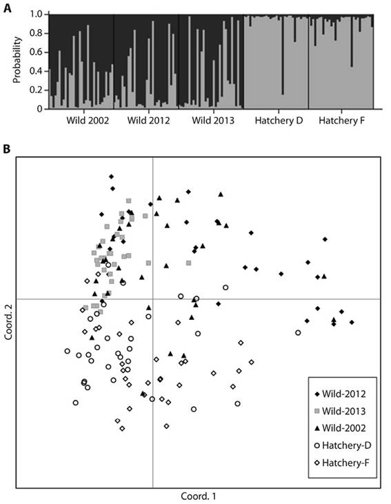
Figure 2 A) Genotypes distribution per sampling site obtained with STRUCTURE software at K = 2. Each column within each location on the horizontal axis represents an individual; thus, the height of the column represents the probability that each individual has a genetic profile of one of the two identified groups. B) Principal Coordinate Analysis of wild and cultivated samples.
Table 4: Individuals with wild origin [Wild-2002 (YAM), Wild-2012 (COL), Wild-2013 (TEC)] assigned to hatchery-origin’s genetic profile with three programsa using 9 loci
| Origin | Test | Mean assignment (%)b | ||
| GenAlEx | Structure | Arlequin | ||
| Wild 2002 (N=32) | YAM-06 | YAM-06 | YAM-06 | 14.7 |
| - | YAM-10 | - | ||
| - | YAM-13 | - | ||
| - | YAM-23 | - | ||
| YAM-24 | YAM-24 | - | ||
| YAM-27 | YAM-27 | YAM-27 | ||
| YAM-30 | YAM-30 | YAM-30 | ||
| Wild 2012 (N=29) | COL-12 | - | - | 6.9 |
| COL-13 | COL-13 | - | ||
| COL-20 | COL-20 | - | ||
| COL-29 | - | - | ||
| Wild 2013 (N=32) | TEC-11 | TEC-11 | - | 7.3 |
| TEC-20 | TEC-20 | - | ||
| TEC-28 | TEC-28 | - | ||
| - | TEC-30 | - | ||
a References for the programs: GenAlEx: Peakall and Smouse (2006, 2012); Structure: Pritchard et al. (2000); Arlequin: Excoffier et al. (2005).
b Mean number of individuals assigned / N * 100.
Discussion
The lack of genetic differentiation among years (2002-2013) indicated that the three locations constitute a single panmictic population. Previous work showed significant genetic differentiation over a wide geographical range from L. vannamei populations along the Eastern Pacific coast (Sunden & Davis, 1991; Valles-Jiménez et al., 2005), but low genetic heterogeneity among lagoons at a regional level in the State of Sinaloa (Perez-Enriquez et al., unpublished data), supporting the hypothesis of a single population in the wild.
When the genetic make-up of hatchery-reared and wild populations was compared, the results of this study indicated significant differences. Based on this, it was suggested that the identification of the origin of individuals using genetic markers is possible. Perez-Enriquez et al. (2009), Mendoza-Cano et al. (2013), and Vela-Avitúa et al. (2013) showed that the genetic composition of hatchery-reared stocks in Mexico is different from wild shrimp most probably due to more than 20 years of domestication and selection, since the establishment in Texas of a synthetic population from Mexico and Central America in the 80’s (Perez-Enriquez et al., 2009).
The deviations from Hardy-Weinberg equilibrium observed in both hatchery-reared and wild samples indicated that either null alleles were present in the analyzed loci and/or one or more of the assumptions of the HWE model were not met.
In the present study, the two loci showing null alleles (Livan13, Livan60) were also recently reported of having this problem in parentage testing (Perez-Enriquez & Max-Aguilar, 2016). It has been recognized that the presence of null alleles may influence the results of population genetic studies (Pompanon, Bonin, Bellemain, & Taberlet, 2005). Nevertheless, the analyses done including these two loci, did not result in a different genetic structure and only a slight difference in the percentage of the assignment pattern (results not shown). This may be explained by the fact that analyses based on allele frequencies are less sensitive to genotyping errors (Pompanon et al., 2005).
In hatchery-reared stocks non-random mating may come from a low effective population size (few broodstock) or kin-ship mating. However, because this is usually not the case in wild populations, it is hypothesized that HWE deviations observed in shrimp samples, could be explained by the Wahlund effect (see Hartl & Clark, 1997) due to population mixing (wild with farmed shrimp). In this regard, HWE deviations were also recorded in wild population samples from five coastal lagoons of Sinaloa (Perez-Enriquez et al., unpublished data). This hypothesis assumes that the genetic composition of hatchery-reared stocks in Mexico has not varied between 2002 and 2013. This is a fair assumption considering that no introductions of broodstock to Mexican hatcheries happened before August 2013 (see http://www.economia-snci.gob.mx/ tariff code 03062701 for Mexican import statistics) and that large population sizes were kept within hatcheries every generation (according to personal communication with several hatchery managers, in Mexico usually more than 1 000 broodstock are used to produce each generation). It also assumed that the genetic composition of the hatcheries D and F, studied here, represented the genetic make-up of all the commercial hatcheries, which is not necessarily true (see Vela-Avitúa et al., 2013).
From our calculations, the proportion of farmed shrimp escaped into the wild varied between 14.7 % in 2002 to an average of 7.1 % in 2012 and 2013. This decrease might be an effect of the location sampled each year (derived from differences of sampling years) or may indicate that the introgression of farm shrimp alleles into the wild has probably been limited.
Intentional or unintentional release of farm shrimp into the wild can come from farms or hatcheries, but there are no data about the number of released individuals. In fish, large numbers of farmed individuals escape every year, e.g. Atlantic salmon in Norway (Taranger et al., 2015) and European seabass in Cyprus (Brown et al., 2015).
In shrimp, escapes may happen during tropical storms. In Northwestern Mexico, tropical storms usually occur from August through October, when shrimps are also harvested. During severe events, rainfall and/or wind may wash away shrimps from farms; in the period 2002-2013 a total of nine hurricanes passed near or through Sinaloa (Comisión Nacional del Agua, (http://smn.cna.gob.mx/index.php?option=com_content&view=article&id=38&Itemid=46), bringing > 60 mm in 24 h to various parts of the state; however, no information is available on the number of shrimp farms that were affected.
Intentional release from hatcheries could be a more important source of farmed shrimps in the wild. During the production season (mainly March through May) hatcheries may have huge numbers of postlarvae that are not sold. A common practice of hatchery managers is to release them, believing that those larvae will survive and benefit the wild population (J. Peiro, Acuacultura Mahr, personal communication). There are no data on the amount of larvae being released, but a rough estimate is 10% of a hatchery’s production (J. Peiro, Acuacultura Mahr, personal communication), which comes to approximately 300-500 million postlarvae per year in the State of Sinaloa. An occasional contribution is the release of larvae as an obliged mitigation measure imposed to farms dredging in estuaries at the farms’ water intakes. It is estimated that since 2009, 500 million larvae have been released (SEMARNAT, personal communication).
Whether escaped shrimp survive or not is not known, but the survival rate will depend on the age, health condition and the environmental and biotic characteristics of the release area (Hamasaki & Kitada, 2006; Wang, Zhuang, Deng, & Ye, 2006). Estimates of survival in stock enhancement programs in Japan of juvenile kuruma shrimp is 0.0-22 % (Hamasaki & Kitada, 2006). Recapture rates of the fleshy prawn in stock enhancement programs in China varied from 0.001-2.0 % (Wang et al., 2006).
The percentage of putatively escaped shrimp of our study, particularly in 2012 and 2013 (3-6 %) is lower than what has been estimated in escapes of the European seabass (15 %; Brown et al., 2015) and the gilthead sea bream (13 %; Šegvić-Bubić et al., 2011). Taranger et al. (2015) suggested that 4-10 % of Atlantic salmon is a moderate introgression risk; however, this estimate is based on the homing behavior of the species. Shrimp in Sinaloa should have a lower risk level, since there does not appear an introgression of hatchery-reared genes occurring in 2012 and 2013, because their genetic make-up is not significantly different from 2002. Nevertheless, the amount of potential introgression will be a function of one-way migration rate (Hartl & Clark, 1997) that in this case, corresponds to the proportion of hatchery-reared organisms respect to wild individuals surviving and reproducing.
The possible genetic impact of aquaculture is a concern in several parts of the world (e.g. Svåsand, Crosetti, García-Vázquez, & Verspoor, 2007; Jacq, Ødegård, Bentsen, & Gjerde, 2011; Kitada et al., 2009), but authors recognize a lack of information in many species and some contrasting results about the genetic effects, which depend on the biology of the species (e.g. behavior, distribution, effective population size), and the region under study. Several examples of the genetic impact of farmed fishes over wild populations were reviewed by Laikre, Schwartz, Waples, Ryman, and The GeM Working Group (2010) in terms of loss of genetic structure (e.g. coho salmon Oncorhynchus kisutch), change in genetic composition (e.g. Adriatic grayling Thymallus thymallus), and adaptation and genetic diversity (e.g. Atlantic salmon). In Japan, changes in genetic diversity or structure of populations under the influx of stock enhancement programs have been reported for the red sea bream Pagrus major (Perez-Enriquez, Takemura, Tabata, & Taniguchi, 2001; Blanco Gonzalez, Aritaki, Knutsen, & Taniguchi, 2015). In contrast, low changes in the genetic composition caused by sea farming or supplementation activities have been reported in wild populations of Atlantic salmon (Glover et al., 2012), the black sea bream Acanthopagrus schlegelii (Blanco Gonzalez, Nagasawa, & Umino, 2008), and the Japanese Spanish mackerel Scomberomorus niphonius (Nakajima et al., 2014). In any case, to what extent genetic structure modifications may impact the fitness of wild populations is a matter of discussion. According to McGinnity et al. (2003) escapees of farmed salmon may reduce the fitness of wild stocks.
In spite of the apparent low-risk levels reported here, management strategies are necessary to avoid release of farmed shrimps into the wild to decrease the probability of gene introgression. Larval release from hatcheries by hatchery managers should be discouraged or stopped; looking for alternative uses, such as food for aquarium fish or fish meal. For stock enhancement, the use of larvae from wild broodstock is recommended (Miller & Kapuscinsky, 2003). At the farms, emergency harvests during the hurricane season could decrease shrimp losses from flooding.

