


 English (pdf)
 Article in xml format
 Article references
 Send this article by e-mail
 Cited by SciELO
  Similars in
SciELO
Similars in
SciELO  uBio
uBio 
 Permalink
The Western Amazon forest, one of the world’s last wilderness areas, supports an extraordinarily high level of species richness across taxa (Bass et al., 2010). However, the increasing levels of human impacts have led to the need to extend nature reserves and apply different types of management regimes, in order to preserve forest biodiversity and dynamics. Besides, forests not included within protection systems, must also be managed in different ways to produce timber and preserve biodiversity (Cañadas, 2005).
Forest structure affects a range of other properties, including biodiversity and habitat functions, and thus the quality of ecosystem services (Gadow et al., 2012). In many parts of the world, forestry objectives have been shifting from focusing on maximum production, to a wider perspective that includes biodiversity preservation and ecosystem functioning (Gadow, 2003). To achieve these targets, managers are increasingly designing cutting regimes that imitate natural disturbances, with the aim of generating more naturally structured forests(Schliemann & Bockheim, 2011).
In many old-growth forests, as ecosystems distinguished by old trees and related structural attributes, tree fall gaps caused by tree death constitute the dominant type of disturbance (Whitmore, 1989). In this context, the concepts of “forest gap” and “gap phase” were introduced by Watt (1947), who used these terms in relation to forest patches created by one or more canopy trees falling. The main causes of canopy gaps in a variety of ecosystems are wind throw, insect damage, disease, acidic deposition, drought and climate change. The application of gap dynamics theory appears to be a promising option for tropical forest management and conservation. However, attempts to manage tropical forest based on these concepts are scarce (Schliemann &Bockheim, 2011).
According to Arriaga (1988), Brokaw and Busing (2000) and Dubé, Fortin, Canham and Marceau (2001), gaps increase light levels and modify local environmental conditions, are required for nearly all tree species to reach canopy status, generate habitats for specific species, become preferential sites of natural regeneration and subsequent growth, form important sites of entry of new genetic variants and new taxa, and may support the existence of some herbivores. Gaps not only help maintain the characteristic uneven-age nature of old-growth forests, but also influence nutrient cycling and preserve soil and plant species diversity (Brokaw & Busing, 2000).
Gap size, age, and distribution are important variables for defining gap status and are strongly associated with gap processes. These variables and other gap characteristics can indicate the regeneration potential for different taxa. A high level of disturbance will result in many gaps or in large gaps. This will lead to a relatively high proportion of species depending on forests gaps (Poorter, Jans, Bongers, & Van Rompaey, 1994). Gap size may be computed by different methods based on two and three dimensional projections of the canopy gap. Gap age can be measured by tree ring analysis, whorl counts and degree of decomposition. At the landscape level, gap processes can be investigated by use of long-term plots, aerial photography, GIS, and increment cores at random points and transects. The processes involved in gap making or infilling can be predicted by several fine and large scale models (Schliemann & Bockheim, 2011).
Currently, various studies on forest gaps attributes are available, but little research has considered the characteristics at gap edges. Understanding natural gap processes is crucial for establishing new forestry practices trying to mimic natural processes of forest disturbance. In the present study, of an old-growth tree species-rich Ecuadorian Neotropical forest, we used multivariate analysis to assess the spatial distribution of gaps and gap size, in relation to tree (stem) number at the gap edge, number of tree species at the gap edge, number of tree species per stem at the gap edge, species similarity at the gap edge, species evenness at the gap edge, size differentiationat the gap edge, gap isolation, and species mingling atthe gap edges.
Material and methods
Site description: The study was conducted in the old-growth forest of the Ávila Viejo community, between October and December 2011. This forest is located in the Province of Orellana, Canton Loreto (0°38’14’’ N & 89°59’6’’ W) and comprises a 3 000 ha tract of old-growth Neotropical forest, in the Protected Forest Sumaco lowland, buffer zone of the National Park Sumaco Napo-Galeras, Ecuador, located at an elevation of 450 m above sea level. The yearly rainfall in the area follows a tri-modal pattern, totalling 4 000 mm.year-1. The mean annual temperature is 24 ºC. The soils, derived from volcanic ash, are alluvial black soils with fine sand, and an irregular distribution of organic material (Cañadas, 1983). No vertebrate studies were carried out, and field work permit was granted by the Ministerio del Ambiente, Ecuador (http://ambiente.gob.ec/).
Field sampling: A 1 ha plot of Neotropical rainforest (the most representative forest of Canton Loreto) was chosen for its flat representative topography. Species, DBH, and the X and Y coordinate for each tree with diameter at breast height (DBH) ≥ 10 cm were measured. Tree botanical species samples were identified by the National Herbarium of Ecuador. The study 1 ha plot was square (100 x 100 m). Every open area (without trees of DBH ≥ 10 cm) was considered to be a “gap” if the opening in the horizontal projection of the canopy over the ground exceeded a predefined minimum area of 9.76 m2(3.12 x 3.12 m) following Brokaw (1982)(Figure 1). General information on gap size, stem number (N), and tree species (S) at the gap edge, according with Muth and Bazzaz (2002) is given in Table 1.
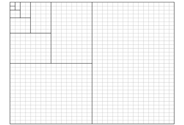
Table 1: Gap size and numbers of species and stems at the gap edge of the one-hectare sampling plot of the tropical rainforest in the Ávila Viejo community, Canton Loreto.
| Gap size (m 2 ) | Number of species | Number of stems | |
|---|---|---|---|
| Minimum | 9.8 | 2.0 | 3.0 |
| Median | 54.1 | 5.6 | 10.4 |
| Maximum | 400.2 | 16.0 | 47.0 |
| Mean (±SD) | 127.4 (± 103.1) | 3.8 (± 2.7) | 7.2 (± 4.9) |
Patterns of gap distribution: Using the agglomerative approach method (AAM) and the Grid2-Simulation program (Vilčko, 2003), two adjacent quadrats (3.12 x 3.12 m), in a 32 x 32 quadrants grid, were combined into blocks of two quadrants, which were in turn successively combined, until a hierarchy of block sizes (r) ranging from 2, 4, 8, 16, …, Kquadrates was obtained (Figure 1). The between-block sums of squares from the block counts in pairs of blocks of sizerthat make up a block of size 2rwere then calculated. The AAM was introduced by Cressie (1993), who analysed contiguous quadrat data by nested analysis of variance. Considering that A i and B i denote the number of events in the ith pair of blocks, each containingrquadrats, the between-blocks sum of squares for blocks (SS r ) was then calculated (Cressie, 1993), as equations 1 and 2:
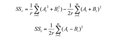
Where:r= block size in number of quadrants; m = K/2r,and the mean square is MSr ≡ SSr/m. Peaks in mean-squares are considered to be associated with a gap size.
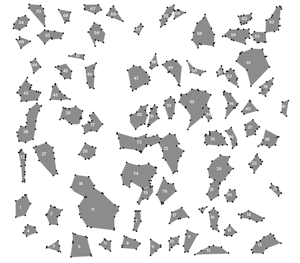
Gap size and isolation: Gap edge and gap polygon were determined using ARC/VIEW 3.2 software (Figure 2). The gap size (GS) and average distance (d i ) between the centre of each gap and other gaps centres provides a measure of gap isolation (I) (eq. 3), where g equals the gap number from Rousseau and VanHecke (1999).
Tree species number: The number of tree species at the edge (S) of each gap was counted and the relationship between gap size and cumulative species number at the gap edges for all gaps surveyed was determined following Muth and Bazzaz (2002). The S per individual tree number at the edges (N) was also calculated to eliminate the area effect on species richness (Hubbell et al., 1999).
Species composition similarity: Species composition similarity at the edge was calculated with the Sørensen coefficient (eq. 4) (Weiner & Solbrig, 1984):
Where Sør = Sørensen coefficient, S c = number of species present at both gap edges (habitats),S a ,S b = number of species present at gap edge A and gap edge B, respectively.
Species evenness: Species evenness at the gap edge was calculated by means of the GINI evenness index (G’) (eq. 5) (Rousseau & Van Hecke, 1999):

Wherep i equals the probability of occurrence of the ith species, and G’= 1 for perfect evenness (p 1 =p 2 …=p s ). The relationship between the gap size and species richness at the gap edge was determined by using a species-gap size curve. The species richness was quantified using the number of species (S) per each gap.
Size differentiation: According to Gadow et al. (2012), size differentiation (U) at the gap edge is defined as the proportion of four neighbouring trees, which are smaller than a given reference tree. This is estimated with equation 6:
Where:v j = 1, if the neighbour is smaller than the reference tree i, and v j = 0 otherwise. If the reference tree has four neighbours, the index U i can have one of five values (0, 0.25, 0.5, 0.75, and 1).
Species mingling:Species mingling at the gap edge and neighbourhood (M i ) was defined as the proportion of trees of different species among the four neighbours of the reference tree (Gadow et al., 2012) (eq. 7):
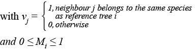
Given four neighbours, the mingling attribute M i can have one of five values (0; 0.25; 0.5; 0.75 and 1).
Principal Component Analysis (PCA):The variables tree number at the gap edge (N), number of tree species at the gap edges (S), number of tree species per stem at the gap edge (S/N), species similarity at the gap edge (Sør), gap size (GS), species evenness at the gap edge (G´), size differentiation at the gap edge (U), gap isolation (I), and species mingling at the gap edge (M), were analysed to detect any relationships between variables using Principal Component Analysis with varimax rotation, and the Spearman correlation index (r s ), by using XLSTAT 2015.1.02 for Windows. The Bartlett test was applied to test the significance of eigenvalues.
Cluster analysis: Cluster analysis is a multivariate procedure that divides the sample into groups that are described by specific characteristics. The goal of this procedure is to form clusters of individuals that are almost homogenous but widely separated from other clusters by their heterogeneity.
In this study, i) the gap attributes N, S, S/N, Sør, GS, G´,U,IandM, along with ii) the algorithms of k-means clustering besides the Calinski-Harabasz criterion and iii) the Affinity Propagation (AP) clustering (with the input preference to the 0, 0.01 and 0.5 quantiles (q) of the input similarities) were used to analyse gap cluster structures. k-means is an iterative, data-partitioning algorithm and requires as input a matrix of points in different dimensions and a matrix of K initial cluster centres in J dimensions, using the Euclidean distance between points and clusters. The general procedure is to search for a K-partition with locally optimal within-cluster sum of squares by moving points from one cluster to another (Hartigan & Wong, 1979).
In contrast with k-means, the AP is a relatively new clustering algorithm that detects exemplars among data points and forms groups of data points around these exemplars. It works by simultaneously considering all data point as potential exemplars and exchanging messages between data points until a set of exemplars and clusters is optimized. AP does not need to be given a pre-defined number of clusters (Frey & Dueck, 2007). The Calinski-Harabasz criterion (sometimes called the variance ratio criterion (VRC)) and an AP search algorithm were used to determine the most suitable number of clusters. The VRC minimize the within-group sum of squares and maximize the between-group sum of squares. The highest VRC value corresponds to the optimal set of most compact clusters (Legendre & Legendre, 2012).
Cluster analyses were performed using the R Script for K-Means Cluster Analysis and “apcluster” software packages (Bodenhofer, Kothmeier, & Hochreiter, 2011) implemented in the free statistical application R (R Core Team, 2014).
Canonical Discriminant Analysis (CDA): Canonical Discriminant Analysis was then used to examine attribute differences between gap clusters detected by cluster analysis (calculated by AP withq= 0.01). The Wilk’s Lambda test was used to check the significance of the clusters defined by AP withq= 0.01, and the Bartlett test was used to test the significance of eigenvalues (Everitt & Dueck, 2001; Polit, 1996). This analysis, including a cross validation was carried out with XLSTAT 2015.1.02 for Windows.
Results
A total of 77 tree species and 811 individuals were recorded at the edges of 78 gaps (in a 32 x 32 quadrant-grid of 3.12 x 3.12 m quadrats). These trees represented 68.7 % of the total number of trees observed in the whole one-hectare studied plot. The total area occupied by all gaps was 4 011 m2/ha. The family and genus of each species represented by individuals in more than 20 % of the gap edges are listed in Table 2. Overall, 1 180 trees were recorded in the one-hectare plot.
Table 2: Tree families and genera found at the gap edges of the one-hectare plot of the tropical rainforest in the Ávila Viejo community, Canton Loreto, Amazonian Ecuador.
| Family | Genus |
|---|---|
| Anacardiaceae | Spondias |
| Anacardiaceae | Tapirira |
| Annonaceae | Guatteria |
| Arecaceae | Iriartea |
| Araliaceae | Schefflera |
| Bignoniaceae | Jacaranda |
| Boraginaceae | Cordia |
| Burseraceae | Dacryodes |
| Burseraceae | Protium |
| Cecropiaceae | Cecropia |
| Cecropiaceae | Pourouma |
| Clusiaceae | Rheedia |
| Clusiaceae | Calophyllum |
| Euphorbiaceae | Alchornea |
| Euphorbiaceae | Hyeronima |
| Fabaceae | Calliandra |
| Fabaceae | Myroxylon |
| Lauraceae | Ocotea |
| Lauraceae | Nectandra |
| Melastomataceae | Miconia |
| Melastomataceae | Mouriri |
| Meliaceae | Guarea |
| Mimosoideae | Inga |
| Moraceae | Ficus |
| Moraceae | Batocarpus |
| Moraceae | Perebea |
| Myristicaceae | Otoba |
| Myristicaceae | Virola |
| Tiliaceae | Apeiba |
| Rubiaceae | Warszewiczia |
| Sapotaceae | Pouteria |
| Sapotaceae | Chrysophyllum |
| Violaceae | Leonia |
The gaps were distributed in a completely spatially random manner in the research plot (Figure 3). In none of the cases the peak mean square occurred in blocks sizes (full line). This result defines a complete spatial random distribution of the gaps in the research plot. The number of new species per unit of gap size remained below 10 % for gap sizes above 127 m2 (Figure 4). This point was considered to be a mean threshold differentiating between small and large gaps. Fifty-eight out of the 78 gaps (74 %) were smaller than 50 m2. Most (70 %) of the tree species found in the whole plot were found at the gap edges.
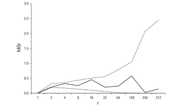
Figure 3 Patterns of gap distribution established using the agglomerative approach method. Mean square MSr (solid line) versus block size r, together with 95% simulation envelopes (dashed lines) for the gaps in one-hectare sample plot. Ávila Viejo community, Canton Loreto.
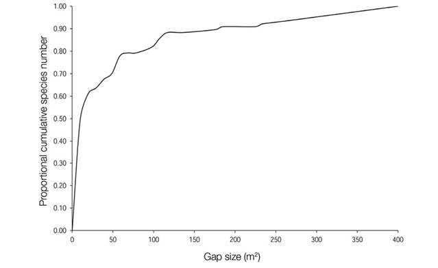
Figure 4 Cumulative number of species at the gap edge-gap size curve for the 78 selected gaps surveyed in the one-hectare plot of tropical rain forest in the Ávila Viejo community, Canton Loreto.
The greater the species mingling in class 0 (see eq. 8), the more different tree species were intermingled. In total, 95 % of the species at the gap edge were surrounded by either four or three neighbours belonging to different species (Figure 5).
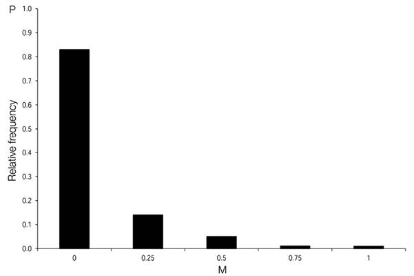
Figure 5 Species mingling distribution (M) of the total gaps surveyed in the Ávila Viejo community, Canton Loreto.
The distribution of size differentiation at the gap edge (U) (Figure 6) was skewed to the left, showing that 35 % of the reference trees were dominant in their immediate vicinity, while most trees (65 %), were surrounded by at least three larger neighbours.
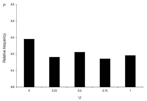
Figure 6 Size differentiation distribution (U) of all gaps surveyed in the Ávila Viejo community, Canton Loreto.
After a varimax rotation, the first three axes of the PCA explained 68.6 % of the total variance (eigenvalues: λ 1 = 3.64, λ 2 = 1.418, λ 3 = 1.31). The Bartlett’s test showed that the eigenvalues of the first three principal components were statistically significantly different from each other (P< 0.0001). Principal component 1 explained the variables number of tree species at the gap edge (S) and total number of individuals at the gap edge (N). The values of N(r s = 0.62), M(r s = 0.68) and G´(r s = 0.73) increased (P< 0.0001) with the size of the gaps (GS). Species richness (S) was strongly positively associated with N(r s = 0.84, P< 0.0001), but not with GS. Principal component 2 elucidated S/N, gap size (GS), species mingling index at the gap edge (M), and species evenness at the gap edge (G´). S/N was negatively correlated with GS(r s = -0.59, P< 0.0001) and M(r s = -0.46, P< 0.0001). Principal component 3 described about 14.5 % of the total variability and defined distribution of tree size differentiation at the gap edge (U) and species similarity at the gap edge (Sør). Gap isolation (I) was not associated with other variables (Figure 7).
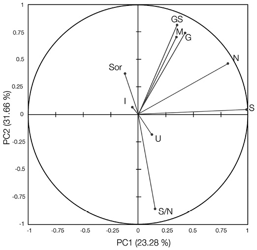
Figure 7 Principal component analysis after varimax rotation for the 78 gaps surveyed in the Ávila Viejo community, Canton Loreto. The component loadings in the two axes (PC1 and PC2) of the centred standardized PCA are shown; GS = gap gize, N = individual number at the gap edge, M = mingling index at the gap edge, I = gap isolation, S/N = number of tree species per stem at the gap edge, G´= species evenness at the gap edge, and S = number of tree species at the gap edge.
After the cluster analysis, the Calinski-Harabasz criterion recommended two clusters as optimal number. The first group comprised the smallest 69 gaps (88 %) and the second group the 9 largest gaps (12 %). The Affinity Propagation (AP) clustering with q= 0 also suggested the same two clusters. Then, AP with q= 0.01 recommended three clusters and with q= 0.5 thirteen groups.
Subsequently a cross validation, the Canonical Discriminant Analysis (Table 3, Figure 8) of the three gap clusters (calculated by AP with q= 0.01) revealed that on average 94.9 % of all gaps were correctly classified. The Bartlett’s test indicated that the eigenvalues of the first two canonical functions were statistically significantly different from each other (P< 0.0001). The Wilk’s Lambda indicated highly significant differences (P< 0.0001) between these three gap clusters. From the first to the third gap cluster, the mean values of gap attributes GS, N, M and S increased monotonically (mean GS from 20 to 232 m2, mean N from six to 29, mean M from 0.16 to 0.47 and mean S from four to eight), but the mean value of S/N decreased from 0.68 to 0.29 (Figure 8). The mean value of the gap isolation (I) was highest in the second cluster (7.5) and lowest in the third cluster (3.8). The mean species evenness at gap edge also was highest in the second cluster (0.95), but lowest in the first cluster (0.87). The distribution of tree size differentiation at the gap edge (U) and species similarity at the gap edge (Sør) varied very little among the three clusters.
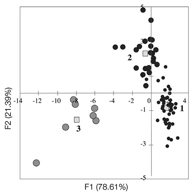
Figure 8 Relationship between three clusters of gaps separated by the Affinity Propagation (AP) clustering with the quantile = 0.01 within a system of two first functions F1 and F2 for the gap community, Ávila Viejo community, Canton Loreto. The squares represent cluster centroids and circles represent gap observations. 1 = the first cluster characterized by the smallest gap sizes, 2 = the second cluster distinguished by the medium gap sizes, and 3 = the third cluster characterized by the largest gap sizes.
Table 3: Variability explained by canonical functions for the seven most important variables (p< 0.0001), that separated three gap clusters detected by the Affinity Propagation (AP) clustering with the quantile = 0.01 within the total canonical structure, in the one-hectare plot of tropical rainforest in Ávila Viejo community, Canton Loreto
| Canonical functions | F1 | F2 |
|---|---|---|
| Eigenvalue | 8.58 | 2.34 |
| Canonical correlation | 0.95 | 0.84 |
| Explained variance | 78.61 % | 21.34 % |
| Variables | ||
| Gap size (GS) | -0.949 | |
| Individual number at the gap edge (N) | -0.921 | |
| Mingling index at the gap edge (M) | -0.794 | |
| Gap isolation (I) | 0.694 | |
| Number of tree species per stem at the gap edge (S/N) | 0.556 | |
| Species evenness at the gap edge (G´) | 0.627 | |
| Number of tree species at the gap edge (S) | 0.501 |
Discussion
The plot that we studied had a density of 1 180 trees/ha. This resulted a similar value to theaverage of 1 387 trees/hareported by Unger, Homeier and Leuschner (2012), for which they evaluated 80 tropical forest plots (0.04 ha) of lowland and lower montane elevations of Amazonian Ecuador (across different edaphic and elevation gradients), close to our research plot, for which they inventoried all trees ≥ 10 cm DBH.
The spatial gap structure in the research plot in the Ávila Viejo community was randomly distributed. However, spatial analysis conducted in the moist forest of Tal National Park in South-West Ivory Coast, West Africa, showed that the occurrence of gaps is often not random, with some sites more likely to have gaps than others places (Poorter et al., 1994). Other studies also suggested that canopy gaps in old-growth Neotropical lowland forests are not spatially randomly distributed, but rather clustered around specific sites such as those with shallow soils (Van der Meer & Bongers, 1996).
The cumulative species-gap size curve showed that 90 % of all species at gap edges were found at the border of the most common group of “small” gaps (≤ 127 m2). These results were similar to those obtained in a study of sapling diversity in an Ecuadorian rainforest, where a threshold of 150 m2was found between small and large gaps. This threshold is an important attribute of the gap distribution (Salvador-Van Eysenrode, Bogaert, Zak-Mnacek, & Ceulemans, 2003). If tree species diversity at gap edges is the main factor influencing tree species diversity in gap regeneration, then the future regeneration in small gaps should also be species-rich. However, in the above-mentioned sapling study, only 30 % of the tree species richness was observed in gaps up to 50 m2 (Salvador-Van Eysenrode et al., 2003). In another study, a sapling species richness of only 21 % was found in gaps smaller than 50 m2 (Hubbell et al., 1999). In these studies, the main causes of species diversity in gap regeneration probably were: i) less adult tree species at the gap edge of small gaps, or/and, ii) an early high degree of species-selective self-thinning, due to intra and inter-specific competition-induced mortality in small gaps, during the course of population development in tree community (Lepš & Kindlmann, 1987; Getzin, Wiegand, Wiegand, & He, 2008; García-Domingo & Saldana, 2013; Wehenkel, Brazão-Protázio, Carillo-Parra, Martínez-Guerrero, & Crecente-Campo, 2015), because of different seed production rate, dispersal, and vigour and shade tolerance of seedlings and saplings of different tree species (Canham, 1989). In contrast, the competition-induced mortality in the larger gaps was probably lower due to lower over story competition on understory gap regeneration.
The low value of the mingling index at the edge of different gaps showed substantial levels of local diversity. The tree species were almost always randomly mixed at the gap border in this one-hectare sample plot, because each tree species was present in a proportion of about 3 % on average. The nearest neighbours were therefore very likely to be of another tree species. This indicates similar capacity among the tree species found to tolerate the abiotic conditions, mainly shade (Kukkonen, Rita, Hohnwald, & Nygren, 2008), and a low potential for competitive niche differentiation in this forest.
The distribution of tree size differentiation was different at the gap edge (U), where most trees were surrounded by at least, three larger neighbours. This type of random distribution can be observed in uneven-aged and mixed forests with a reverseJ-shaped DBH distribution and extremely small minimum balanced structure areas (BSA) and very low minimum balanced structure tree numbers (BSN) (Wehenkel, Corral-Rivas, Hernández-Díaz, & von Gadow, 2011).
The results demonstrated that gap sizes up to 50 m2were mostly sufficient to generate tree species-rich forest stands. In a previous study, gaps were found to vary in size between 20 and 705 m2in a tropical rainforest in Panama (Brokaw, 1985). In other large studies, 70 % of gaps were smaller than 50 m2, and only 0.7 % of all the 1 284 studied gaps were equal or larger than 400 m2in a tropical forest (Panama) (Hubbell et al., 1999), while only 4 % of the gaps exceeded 500 m2in a rainforest in Costa Rica (Sanford, Braker, & Hartshorn, 1986). Another study of 250 000 trees in Panama demonstrated that only 5 % of these trees were adapted to treefall gaps (Welden, Hewett, Hubbell, & Foster, 1991). In contrast, in our study, the gaps were no larger than 400 m2in the one-hectare sample plot. Therefore, if the aim of forest management is to keep the current species composition and biodiversity, logging gaps should preferably be no larger than 400 m2. This corresponds to a selective logging of maximum two neighbour large trees at a time. A mean gap size of 181 m2by conventional selective logging of one single tree and 355 m2by the logging of two neighbouring trees was reported for a tropical rainforest in Guyana (Dam, 2001). Besides, the authors of the same study also showed that nutrient availability is strongly associated with gap size (Dam, 2001).
The PCA analysis confirmed that the lack of correlation between gap size and isolation might be stochastic (see also Salvador-Van Eysenrode et al., 2003). The dense gap grid of 78 mostly small gaps per hectare may provide optimal conditions for regeneration of shade-tolerant tree species, for which dispersal is limited due to large seed size (Canham, 1989).
In this study, relationships between other important characteristics of forest gaps were also observed. Tree species evenness, species and tree number at the edges of larger gaps were highest, probably due to a simple area effect (Hubbell et al., 1999). However, the number of tree species per stem at the edges (S/N) of the largest gaps was significantly lower than that at the smaller gaps. Thus, the number of tree species per stem could control the gap size and influence resistance and resilience of the spatial tree structure in the plot (Gregorius, 2001; Kennedy et al., 2002).
Different tree species often have different life spans and sizes. Therefore, the probability that two or more trees of different species fall at the same time and create a gap is lower than for trees of the same species. Furthermore, the edges of small gaps probably provide more potential regeneration diversity or/and more niches than edges of large gaps, because of the better distribution of shadow and light. Therefore, niche differentiation in response to small changes in understory light may be an important factor in preserving intra habitat diversity (Svenning, 2000). Our finding contrasted with the non-significant to positive relationship between gap size and tree species number per stem, reported in another study (Hubbell et al., 1999). Forest gaps generally promote larger species richness, although usually by sustaining higher stem densities and not by providing more niches (Brokaw & Busing, 2000).
Natural disturbances that create gaps in the canopy are important for stability, heterogeneity (species diversity), turnover rate, and spatial structure in Neotropical forests (Cañadas, 2005). Information about the characteristics of such gaps is therefore crucial for understanding the ecological performance of a forest. Such information can also be used to establish sustainable forest management systems (Wehenkel, Corral-Rivas, & Gadow, 2014). Assuming that our results were representative for an old-growth neotropical rainforest in Ecuador, our study has allowed us to remark the following management recommendations: 1) This rainforest type has a very complex spatial and diversity structure; therefore, logging activities should preferably be omitted, since they will adversely affect these structures. 2) If logging is inevitable, then this intervention should mimic the structures found in this study, i.e., i) a random choice of tree species and sizes to be harvested, avoiding special selection of tree dimension and species, ii) a random distribution of trees to be logged, producing gaps commonly smaller than 50 m2and never larger than 400 m2. Furthermore, we suggest cutting not more than 5 % of the tree biomass in each period of 10-20 years, to preclude stronger alterations of ecosystem processes, and the reduction of existing dead wood into the ecosystem.

