


 English (pdf)
 Article in xml format
 Article references
 Send this article by e-mail
 Cited by SciELO
  Similars in
SciELO
Similars in
SciELO  uBio
uBio 
 Permalink
Introduction
In South America, the Paraná River Delta is an important island and wetland ecosystem composed of groups of islands interconnected and separated by water courses. It is characterized by a high environmental heterogeneity driven by current fluvial activity, as well as historical components (geomorphology of the early Neogene, different flow intensities, marine ingressions, and Pleistocene aeolian processes). All these factors have generated a diverse and dynamic habitat structure, both at spatial and temporal scales. This system is in constant activity, with regular flood pulses of different magnitude and intensity that generate a macrosystem of wetlands in the lower Paraná River (Naiman et al., 2005; Neiff & Malvárez, 2004). These features depend on the water level at a given time and influence the island geomorphology and biology, contributing to the landscape heterogeneity (Beltzer & Quiroga, 2007; Lorenzón, 2014).
Islands comprising these wetland systems exhibit distinctive vegetation that colonizes the territory by seed dispersal in various ways. Seeds are dispersed by anemochory, endozoochory (internal dispersal by fauna), epizoochory (external dispersal by fauna), by certain non-standard dispersal vectors due to alternative morphologies of seed diaspores (Heleno & Vargas, 2015) and through hydrochory (through river courses) (Kubitzk & Ziburski, 1994). All these mechanisms operate together to generate the vegetation of the wetland system, which in turn is different from that of the continent.
Associated with the particularity of the vegetation of the wetland system, the bird communities in the floodplain of the Paraná River behave differently than those in other areas, such as higher topographic areas, which are not directly influenced by the river (Ronchi-Virgolini et al., 2011). Besides the environmental variability mediated by seasonality, there are also the temporal dynamics of the seasonal pulse (Lima et al., 2021; Ronchi-Virgolini et al., 2008; Tockner et al., 2000a). In fluvial forests, vertical stratification of the vegetation provides structural complexity, which allows the occurrence of greater bird richness, abundance and diversity than in the surrounding areas, as well as the provision of protection, nesting and feeding sources (Anjos et al., 2007; Di Giacomo & Contreras, 2002; Giraudo & Ordano, 2003; Lima et al., 2021).
Several studies exploring bird communities in fluvial systems have shown the impact of spatial heterogeneity of vegetation on avifauna. These investigations entailed comparisons of bird assemblages across diverse environmental units on levees, including wetlands, forests, and grasslands (Beltzer & Neiff, 1992; Berduc et al., 2015; Frutos et al., 2020a, Frutos et al., 2020b; Lorenzón et al., 2016; Lima et al., 2021; Ronchi-Virgolini et al., 2010; Ronchi-Virgolini et al., 2011; Ronchi-Virgolini et al., 2013; Rossetti & Giraudo, 2003). Additionally, studies specifically delved into the distinctions between bird communities in upland forests (located outside flood-prone areas) and levee forests, treating these as contrasting environmental units (Ronchi-Virgolini et al., 2011).
Spatial heterogeneity plays a crucial role in shaping bird communities. Changes in bird communities, such as population density, species richness and dominant species composition, have been attributed to variations in forest vegetation conditions, water supply to floodplains and the density of population in different areas of the landscape (Gureev et al., 2019). In addition to hydrological disturbances on floodplains, latitudinal changes along rivers coupled with local habitat characteristics contribute to shaping the conditions that influence bird to habitat affinities (Munes et al., 2015). The intrinsic characteristics of river microenvironments change along the water corridors and are not transferable between regions (Miller et al., 2004), highlighting the unique micro-environmental heterogeneity of each region. Different responses have previously been proposed in relation to the variation in bird assemblages for anthropically intervened riparian environments, depending on the changes generated in spatial heterogeneity (Hernández-Belloso et al., 2018; Martin & Possingham, 2005; Rannestad et al., 2015; Velásquez-Valencia, 2018).
Silvopastoral and agroforestry environments generate patches of dense vegetation with greater richness and diversity of species, such as those reported for Amazonian riparian systems (Velásquez-Valencia, 2018). On the contrary, livestock pressure would compete with bird resources in the lower strata, generating a decrease in bird species (seen in the Australian riparian system) (Martin & Possingham, 2005).
Some environments that have been recovered have exhibited greater associated heterogeneity, thus hosting the greatest diversity of birds, or have demonstrated greater richness and relative abundance. Reported examples include the Kilombero Valley in East Africa (following recent livestock removal) (Rannestad et al., 2015) and Spanish lake environments undergoing restoration (Hernández-Belloso et al., 2018).
Considering that levee forests differ in the structure and composition of the vegetation (Aceñolaza et al., 2005), we focus on evaluating the differences in the structure of the levee forest and how it would affect the bird communities of the Paraná basin. In this work, we focus on differences in bird assemblage between environments within an environmental unit, in our case the floodplain levee forest. We hypothesize that birds use the different levee types differently and that this variation in the use is reflected in the bird assemblage structure within each forest.
Materials and methods
Study area: The study sites included Wetlands in the Pre-Delta National Park (PDNP), Diamante, Entre Ríos, Argentina (32º 03’43” S & 60º38’39” W) (PDNP, 2022) and in the Islas de Santa Fe National Park (ISFNP), San Jerónimo, Santa Fe, Argentina (32°6’10.70”-32°19’42.18” S & 60°43’52.36”-60°36’7.42” W) (Fig. 1) (ISFNP, 2022). These wetland areas correspond to the Delta e Islas del Paraná ecoregion (Matteucci, 2012; Quintana & Bó, 2010). They conform to the Ramsar site ‘Paraná Delta,’ a globally significant wetland located in Argentina (Giacosa et al., 2019). Located in a transition segment in the Paraná River, it is the area where the delta system begins, and is influenced by the biota present in the previous section of this river, the segment called middle Paraná (Lorenzón et al., 2019; Nestler et al., 2007; Sabattini & Lallana, 2007).
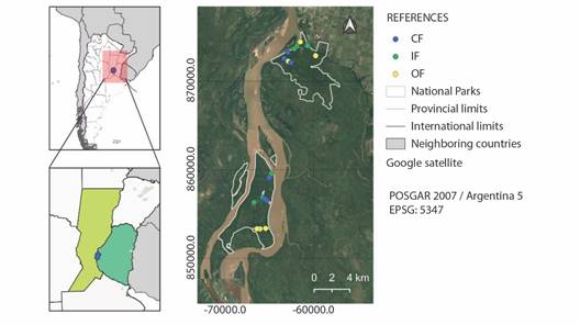
Fig. 1 Map of the study area. The lower polygon represents the limit of the Islas de Santa Fe National Park (ISFNP) and the upper polygon represents the limit of the Pre-Delta National Park (PDNP). Points represent the vegetation sampling points and bird count points (OF= open forests, IF= intermediate forests, CF= closed forests).
The Pre-Delta National Park (PDNP) covers 2 458 hectares of island area and has been under the jurisdiction of the National Parks Administration since 1992. This is the only IBA (Important Bird and Biodiversity Conservation Area) located in the Upper Delta, in the area called “Forests, prairies and meander floodplains” (Coconier & Di Giacomo, 2009). The Islas de Santa Fe National Park (ISFNP) was created in November 2010. It covers 4 096 hectares, including eight islands that have been under the jurisdiction of the National Parks Administration since 2010 (https://www.argentina.gob.ar/parquesnacionales).
Levee forests are located at the highest zone of the floodplain. They have characteristics due to their topographic position, susceptible to floods (Aceñolaza et al., 2004). These forests cover about 20 % of the island area (Borodowski, 2006), whereas the central zones of the islands hold marshes and ponds. In the Paraná Delta, levees are simple, low diversity and open canopy forests, composed of high colonizer trees dominated by Salix humboldtiana and Tessaria integrifolia, with possible occurrence of Albizia inundata, Erythrina crista-galli or Sapium haematospermum. There are mature and better preserved forests (of equal ages) with one or two vegetation strata composed of Nectandra falcifolia and Inga uraguensis, Vachellia caven, and Croton urucurana. There may also be Morus spp. and Ligustrum lucidum as invasive introduced species as a result of ornithochorous dispersal (Ronchi-Virgolini et al., 2010). These forests are complemented by an herb stratum, composed of short gramineous species and grasslands of different species, and a shrub stratum characterized by several vines, sapling and medium-sized trees of Myrsine laetevirens and Zanthoxylum fagara (Aceñolaza et al., 2004; Aceñolaza et al., 2005; Beltzer & Neiff, 1992).
Climate and biogeography: The climate is temperate/warm humid (Kottek et al., 2006). The annual average temperature is about 19 ºC and annual rainfall is ~900 mm, with warmer and rainier summer periods than in winter. Biogeographically, the subtropical biota reaches the temperate zone of the Paraná Delta through the Paraná River, which acts as a biological corridor of great latitudinal extension (Cabrera, 1994; Malvárez, 1999). Thus, the area holds floristic components of the Amazonian domain (with elements from the Paranaense province) and the Chaco domain (with elements from the Chaco, Pampean and Espinal provinces), both domains belonging to the Neotropical Region (Cabrera, 1994); fauna with components of the Mesopotamian District (Subtropical Domain, Guyana-Brazilian subregion) with influence of the Pampean District (Ringuelet, 1961), and overlap of three ornithogeographic zones: the Paranaense province (Forests district) and the Mesopotamian and Pampean provinces (Nores, 1987).
Experimental design for vegetation: The forest types were defined by visually determining the tree cover percentage (on a horizontal plane), in sampling units, following Matteucci & Colma (1982). The area of the vegetation sample points coincided with the area of the bird count points. All the studied forests were considered levee forests because they are present in the highest zone, on the island edges, within the floodplain, without discriminating between young or mature forests, with greater or lower susceptibility to hydrometric fluctuations (Neiff, 2005; Placci, 1994).
A total of 18 vegetation and bird communities sampling points were selected; they were determined according to the vegetation traits (physiognomic-structural categories). Six replicates homogeneously distributed in both national parks were established for each forest category (three replicates in each forest type for each park) (Fig. 1). Forest characterizations based on tree cover ranges were up to 30 % for open forests, between 30 % and 60 % for intermediate forests, and more than 60 % for closed forests (Symonds & Johnson, 2008) (Fig. 2). Percent cover of shrub and herb strata was also recorded, as well as height (cm) of herb stratum.
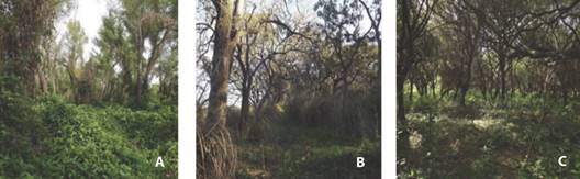
Fig. 2 Physiognomy of the different levee forests. A. Open forest. B. Intermediate forest. C. Closed forest.
Experimental design for birds: Bird sampling was conducted twice in each season, in the same points used for vegetation, at 45-day intervals for three years (2014, 2015 and 2016) and under favorable climatic conditions for bird observation. Birds were counted using the point counting method. To ensure sample independence, distance between points was greater than 250 m. All the birds in the forest environment seen and heard at each point for ten minutes were recorded (Blake, 1992; Ronchi-Virgolini et al., 2011). The total sampling effort at each point was four hours throughout the entire sampling period. This means that in each type of forest, in each park, the total sampling effort during the three years was 12 hours (given the three counting points for each forest type located in each of the two parks). All the birds that made use of the habitat were recorded, except for those that were seen only flying over the area. The estimated radius of the count point was 75 m. Counts began at sunrise and continued for four hours, the period of greatest stability for bird detection (Huff et al., 2000; Ralph et al., 1996). On each visit, sampling order was shifted among points to reduce the effects associated with bird activity and time of the day (Verner & Milne, 1989). All the species were identified in situ (Narosky & Yzurieta, 2010) and then classified systematically according to SAAC (Remsen et al., 2022).
Sample processing: The bird community was analyzed for each season from the 18 samples homogeneously distributed between the different forest types in both national parks, using a balanced and complete sampling design (Quinn & Kough, 2002). The total observation time for each type of forest was 24 hours during the entire study period, contemplating all points between the two parks, with 6 hours allocated to each season. To obtain more representative estimations of the bird community, seasonal estimates made across three years were grouped in a single point; thus, each sample resulted in the sum of six (6) individual estimates made for each point.

Where P is the sampling point, i is each estimation of bird counts made from a seasonal sampling, and N is the number of terms of the sum or the total estimations throughout the sampling. Bird richness and abundance, species composition and diversity were determined to describe the community structure of each forest type. Diversity was calculated using the Shannon and Weaver diversity index (H´).
Statistical analysis: Composition and relative abundances of tree species were analyzed using an analysis of similarities (ANOSIM) (Clarke & Warwick, 2001) and a non-metric multidimensional scaling (NMDS) (McCune & Mefford, 1999), with the Vegan package (Oksanen, 2011), using the Bray Curtis dissimilarity index on a matrix of relative abundances. Differences in tree, shrub and herb cover among seasons and between sites, and physiognomic differences inherent to forests (forest types) were analyzed using the Kruskall-Wallis non-parametric test (α = 0.05).
The relationship between bird community structure (richness, abundance and diversity) and forest type and sites were evaluated using generalized linear models for each season (Supplementary Material SM1). The models were fitted with the error distribution assumed according to the nature of the data, considering under and/or overdispersion (Gaussian, Poisson and Negative Binomial). Assumptions were evaluated for each model with their residuals (homoscedasticity and normality of Gaussian distribution and under and/or overdispersion in Poisson or Negative Binomial distributions).
Models were selected using the Akaike Information Criteria, as recommended for small samples (AICc) (Burnham et al., 2011; Matthew & Moussalli, 2011). When the best model was not achieved, the multiple model inference (MMI) of those with a Δi < 2 (Matthew & Moussalli, 2011) was used to obtain the relative importance of each predictor variable. The software packages R Studio version 3.6.1 (R Core Team, 2019) and R-medic (Mangeaud & Elías-Panigo, 2018) were used. Response variables whose explanatory variables were statistically significant are reported in Table 2 and Table 3. The figures were done with package Ggplot2 and the editing was done with Corel Draw 2021.5 Licence Adriana Manzano.
Results
Vegetation structure: The analysis of tree composition and relative abundance using the similarity analysis (ANOSIM) and the multidimensional ordination (NMDS) allowed us to differentiate three groups of forests and to associate Tessaria integrifolia and Salix humboldtiana with open forests, Albizia inundata, Myrsine laetevirens, Sapium haematospermum, Enterolobium contortisiliquum, Inga uraguensis and Vachellia caven with intermediate forests, and Erythrina crista galli, Nectandra falcifolia, Croton urucurana and Ligustrus lucidum with closed forests (ANOSIM R = 0.59, P = 0.001; Fig. 3).
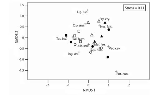
Fig. 3 Non-metric multidimensional scaling (NMDS) of relative abundance of tree species in 18 count points. In black empty symbols, points of the Pre-Delta National Park site; in black filled symbols, points of the Islas de Santa Fe National Park. Open, intermediate, and closed forests are represented by squares, circles and triangles, respectively. Red crosses symbols stand for the relative positions of the different tree species. Tes.int.: Tessaria integrifolia; Sal.hum.: Salix humboldtiana; Alb. inu.: Albizia inundata; Myr. lae.: Myrsine laetevirens; Sap. hae.: Sapium haematospermum; Ent. con.: Enterolobium contortisiliquum; Ing. ura.: Inga uraguensis; Vac. cav.: Vachellia caven; Ery. cri.: Erythrina crista galli; Nec. fal.: Nectandra falcifolia; Cro. uru.: Croton urucurana; Lig. luc.: Ligustum lucidum.
Regarding vegetation cover, no seasonal variation was recorded in tree or shrub cover. The herb stratum showed variation in spring, with its cover being the highest of all seasons (H = 36.77, P < 0.001). The height of this stratum was lowest in winter and highest in spring (H = 29.74, P < 0.001), with no differences between autumn and summer. No differences in cover were detected in any stratum, showing homogeneity in the values of both sites (Fig. 4 and Fig. 5). Regarding the inherent levee forest structure, three physiognomies were detected in the levee forests: open forests (OF), intermediate forests (IF), and closed forests (CF), which were determined by the tree cover (H = 42.52, P < 0.001) and height of the herb stratum (H = 18.69, P < 0.001). In the OF, the lowest tree cover percentage and the highest herb height were recorded. In the IF, both variables had intermediate values, and in CF, the highest percentage of tree cover, and the lowest percentage of herb cover were recorded (Fig. 6.A and Fig. 6.D; Table 1). While tree cover and herb height determined three forest physiognomies, in IF shrub cover was the highest, with no differences between OF and CF (H= 34.71, P < 0.001). The OF herb stratum cover was the highest, with no differences between the IF and the CF (H = 6.97, P < 0.05) (Table 1) (Fig. 6B, Fig. 6C).
Table 1 Differences among vegetation strata with respect to seasons, sites and forest types.
| Dependent variable | Explanatory variable | Statistical (H) | P |
| Tree cover | Season | 0.44 | 0.930 |
| Shrub cover | Season | 0.01 | 0.990 |
| Herbaceous cover | Season | 36.77 | < 0.001* |
| Herbaceous height | Season | 29.74 | < 0.001* |
| Tree cover | Site | 1.67 | 0.199 |
| Shrub cover | Site | 3.61 | 0.060 |
| Herbaceous cover | Site | 3.42 | 0.060 |
| Herbaceous height | Site | 0.62 | 0.430 |
| Tree cover | Forest type | 42.52 | < 0.001* |
| Shrub cover | Forest type | 34.71 | < 0.001* |
| Herbaceous cover | Forest type | 6.97 | 0.030 * |
| Herbaceous height | Forest type | 18.69 | < 0.001* |
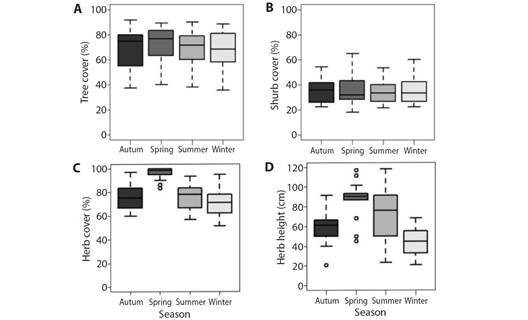
Fig. 4 Seasonal changes in the cover of the different vegetation strata. A. Percentage of tree cover. B. Percentage of shrub cover. C. Percentage of herb cover. D. Height of herb stratum.
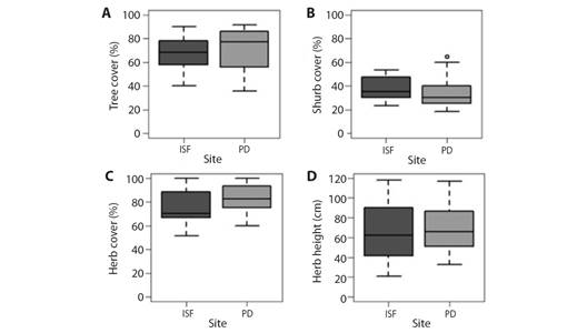
Fig. 5 Differences in cover of vegetation strata between national parks. A. Percentage of tree over. B. Percentage of shrub cover. C. Percentage of herb cover. D. Height of herb stratum.
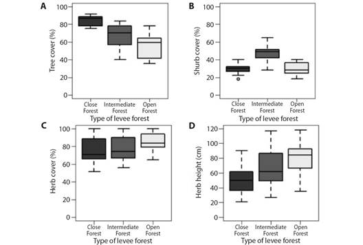
Fig. 6 Intrinsic physiognomic differences among levee forests are determined by percentage of tree, shrub and herb cover, and height of herb stratum. Open forests (OF), intermediate jDifferentiation of shrub cover percentage. C. Differentiation of herb cover. D. Differentiation of herb stratum height (cm).
The results of the Kruskall-Wallis tests are shown.
Bird community: The number of contacts with birds recorded amounted to 9 908, corresponding to 85 bird species belonging to 29 families and 13 orders (Table 3). In autumn, 37.61 % of variation in species richness was explained by physiognomic variables of levee forests (AICc = 104.50, w = 0.60), with OF having higher values than CF (P < 0.01). In spring, richness had the lowest value in PDNP and varied among forest types, with CF showing the lowest value and differing from OF and IF (P < 0.05). In summer, richness had the lowest value in PDNP and varied among forest types with differences between IF and CF. IF had higher richness than CF (P < 0.01). In winter, richness was similar among forest types (Table 2, Table 3, Fig. 8).
Table 2 Seasonal variation in bird richness, abundance and diversity, related to levee forest structure.
| Dependent Variable | AICc | delta | Weight | Coeficient | Coef.Standard deviation | Confidence interval | p-value | Null deviance | Residual deviance | Devianza | Mean ± sd | ||
| Explanatory variable | 2.50 % | 97.50 % | |||||||||||
| Winter Richness | MMI | -0.344 | 0.235 | PDNP site | -0.842 | 0.153 | 0.175 | - | - | - | - | ||
| Autumn Richness | 104.50 | 2 | 0.57 | 35.333 | 1.452 | Open forests* | 32.49 | 38.18 | < 0.01 | 304.00 | 189.67 | 37.61 | 35.33 ± 3.01 |
| -6.167 | 2.053 | Closed forests* | -10.19 | -2.14 | < 0.01 | 29.17 ± 3.60 | |||||||
| Spring Richness | MMI | -0.518 | 0.192 | Closed forests* | -0.93 | -0.11 | 0.01 | 39.17 ± 4.71 | |||||
| -0.641 | 0.178 | PDNP site* | -1.02 | -0.26 | < 0.01 | 38.78 ± 3.89 | |||||||
| Summer Richness | MMI | -3.633 -5.674 | 1.506 1.506 | Intermediate forests* Closed forest* | -1.05 -1.11 | -0.01 -0.06 | < 0.05 < 0.05 | 35.17 ± 3.31 34.67 ± 3.20 | |||||
| Winter Abundance | 160.30 | ~2 | 0.59 | -0.142 | 0.042 | PDNP site* | -0.26 | -0.02 | < 0.05 | 23.53 | 18.00 | 23.49 | 122 ± 12.38 |
| 4.947 | 0.060 | ISFNP site* | 4.87 | 5.03 | < 0.01 | 141 ± 22.06 | |||||||
| Autumn Abundance | MMI | -0.005 | 0.002 | Closed forests* | -0.01 | 0.00 | < 0.05 | 114 ± 13.70 | |||||
| Spring Abundance | 145.10 | > 2 | 0.77 | 5.171 | 0.025 | ISFNP site* | 5.12 | 5.22 | < 0.01 | 34.26 | 15.60 | 54.46 | 176 ± 12.83 |
| -0.160 | 0.037 | PDNP site* | -0.23 | -0.09 | < 0.01 | 150 ± 12.37 | |||||||
| Summer Abundance | MMI | -0.003 | 0.001 | Intermediate forests* | -0.01 | 0.00 | < 0.05 | 126 ± 17.85 | |||||
| -0.004 | 0.001 | PDNP site* | -0.01 | 0.00 | < 0.01 | 122 ± 15.80 | |||||||
| Winter Diversity | -26.60 | ~2 | 0.67 | 3.328 | 0.041 | Open forests* | 3.25 | 3.41 | < 0.01 | 0.24 | 0.10 | 56.76 | 3.26 ± 0.13 |
| -0.157 | 0.050 | Closed forests* | -0.26 | -0.06 | < 0.01 | 3.11 ± 0.07 | |||||||
| 3.328 | 0.041 | ISFNP site* | 3.25 | 3.41 | < 0.01 | 3.25 ± 0.10 | |||||||
| -0.118 | 0.041 | PDNP site* | -0.20 | -0.04 | < 0.05 | 3.13 ± 0.11 | |||||||
| Autumn Diversity | MMI | -0.962 | 0.375 | Closed forests* | -1.73 | -0.19 | < 0.05 | 3.16 ± 0.13 | |||||
| 0.895 | 0.285 | Closed forests in PDNP site* | 0.27 | 1.52 | < 0.01 | 3.18 ± 0.06 | |||||||
| Spring Diversity | -28.10 | > 2 | 0.77 | 3.590 | 0.039 | Open forest* | 3.51 | 3.67 | < 0.01 | 0.26 | 0.10 | 63.08 | 3.58 ± 0.05 |
| -0.122 | 0.048 | Intermediate forests* | -0.22 | -0.03 | < 0.05 | 3.40 ± 0.10 | |||||||
| -0.144 | 0.048 | Closed forests* | -0.24 | -0.05 | < 0.01 | 3.37 ± 0.14 | |||||||
| 3.590 | 0.039 | ISFNP site* | 3.51 | 3.67 | < 0.01 | 3.50 ± 0.10 | |||||||
| -0.143 | 0.039 | PDNP site* | -0.22 | -0.07 | < 0.01 | 3.36 ± 0.11 | |||||||
| Summer Diversity | MMI | -0.629 | 0.244 | Closed forests* | -1.15 | -0.11 | < 0.05 | 3.24 ± 0.06 | |||||
Seasonal variation in the community attributes related to forests structure. MMI: Multiple Model Inference. PDNP: Pre-Delta National Park. ISFNP: Islas de Santa Fe National Park. AICc value (small samples), delta and weight of the best model, coefficient value and standard deviation, confidence interval and P of the explanatory variables (*significance).
Table 3 Systematic classification of bird species in each site, their richness and number of contacts of each one.
| Species | Status | ISFNP | PDNP | ||||||||||||
| Conservation | Richnnes | Number of Contacts | Richnnes | Number of Contacts | |||||||||||
| OF | IF | CF | OF | IF | CF | OF | IF | CF | OF | IF | CF | ||||
| Hydropsalis torquata* | LC | - | - | X | - | - | 1 | - | - | - | X | - | - | 1 | |
| Butorides striata | LC | - | - | - | X | - | - | 1 | X | X | X | 1 | 1 | 1 | |
| Columbina picui | LC | - | X | - | - | 2 | - | - | X | X | - | 2 | 4 | - | |
| Columbina talpacoti | LC | | X | - | - | 1 | - | - | X | X | X | 5 | 1 | 2 | |
| Leptotila verreauxi | LC | - | X | X | X | 62 | 85 | 95 | X | X | X | 105 | 142 | 155 | |
| Patagioenas maculosa | LC | | X | - | - | 1 | - | - | - | - | - | - | - | - | |
| Patagioenas picazuro | LC | | X | X | X | 39 | 53 | 61 | X | X | X | 60 | 75 | 74 | |
| Zenaida auriculata | LC | | X | X | X | 33 | 44 | 24 | X | X | X | 28 | 17 | 9 | |
| Chloroceryle amazona | LC | X | - | X | 1 | - | 1 | - | X | - | - | 2 | - | ||
| Chloroceryle americana | LC | X | - | X | 2 | - | 2 | X | X | - | 1 | 3 | - | ||
| Megaceryle torquata | LC | - | X | - | X | 1 | - | 1 | - | X | - | - | 3 | - | |
| Coccycua cinérea* | LC | X | X | - | 3 | 1 | - | X | - | - | 1 | - | - | ||
| Coccyzus melacoryphus* | LC | - | X | X | X | 4 | 1 | 4 | X | X | X | 2 | 2 | 3 | |
| Guira guira | LC | | X | X | X | 4 | 2 | 10 | - | X | X | 1 | 4 | 2 | |
| Tapera naevia* | LC | - | X | - | - | 1 | - | - | X | - | - | 2 | - | - | |
| Rostrhamus sociabilis | LC | - | X | - | - | 1 | - | - | - | X | X | - | 1 | 1 | |
| Rupornis magnirostris | LC | X | X | X | 17 | 13 | 14 | X | X | X | 7 | 4 | 13 | ||
| Caracara plancus | LC | | X | X | X | 8 | 5 | 5 | X | X | X | 19 | 6 | 9 | |
| Aramus guarauna | LC | - | - | - | X | - | - | 1 | - | - | - | - | - | - | |
| Aramides ypecaha | LC | - | X | X | - | 3 | 2 | - | - | - | - | - | - | ||
| Campylorhamphus trochilirostris | LC | X | X | X | 1 | 6 | 1 | X | X | X | 6 | 4 | 5 | ||
| Lepidocolaptes angustirostris | LC | | X | X | X | 89 | 43 | 54 | X | X | X | 68 | 52 | 69 | |
| Microspingus melanoleucus | LC | - | X | X | X | 44 | 15 | 7 | X | X | X | 11 | 7 | 5 | |
| Saltator aurantiirostris | LC | Unk | X | X | X | 66 | 80 | 76 | X | X | X | 74 | 71 | 69 | |
| Saltator coerulescens | LC | X | X | X | 124 | 162 | 134 | X | X | X | 126 | 114 | 125 | ||
| Saltator similis | LC | - | X | - | - | 1 | - | - | - | - | - | - | - | ||
| Paroaria capitata | LC | - | X | X | X | 45 | 26 | 45 | X | X | X | 22 | 5 | 8 | |
| Paroaria coronata | LC | - | X | X | X | 27 | 24 | 23 | X | X | X | 25 | 13 | 17 | |
| Poospiza nigrorufa | LC | - | - | X | X | - | 2 | 2 | X | - | X | 3 | - | 2 | |
| Sicalis flaveola | LC | - | X | X | X | 6 | 9 | 2 | X | X | X | 4 | 8 | 4 | |
| Zonotrichia capensis | LC | - | X | X | X | 30 | 35 | 47 | X | X | X | 16 | 9 | 22 | |
| Spinus magellanicus | LC | - | X | X | X | 16 | 1 | 2 | X | X | - | 12 | 4 | - | |
| Asthenes pyrrholeuca** | LC | X | X | X | 6 | 10 | 4 | - | - | - | - | - | - | ||
| Certhiaxis cinnamomeus | LC | X | X | - | 2 | 2 | - | X | - | - | 1 | - | - | ||
| Phacellodomus ruber | LC | X | X | X | 139 | 111 | 156 | X | X | X | 148 | 127 | 134 | ||
| Phacellodomus striaticollis | LC | - | X | X | - | 1 | 1 | - | - | - | - | - | - | - | |
| Synallaxis frontalis | LC | X | X | X | 36 | 56 | 39 | X | X | X | 34 | 57 | 43 | ||
| Limnoctites sulphuriferus | LC | X | X | X | 1 | 2 | 4 | - | - | - | - | - | - | ||
| Furnarius rufus | LC | X | X | X | 56 | 70 | 66 | X | X | X | 53 | 48 | 62 | ||
| Progne tapera* | LC | X | X | X | 38 | 14 | 18 | X | X | X | 35 | 24 | 19 | ||
| Tachycineta leucorrhoa | LC | | X | X | X | 55 | 31 | 17 | X | X | X | 27 | 13 | 16 | |
| Agelasticus cyanopus | LC | - | X | X | X | 3 | 8 | 5 | X | X | - | 2 | 2 | - | |
| Cacicus solitarius | LC | - | X | X | X | 4 | 17 | 5 | X | X | X | 14 | 9 | 23 | |
| Icterus pyrrhopterus | LC | - | X | X | X | 28 | 10 | 18 | X | X | X | 18 | 13 | 13 | |
| Agelaioides badius | LC | - | X | X | X | 52 | 54 | 39 | X | X | X | 26 | 39 | 23 | |
| Molothrus bonariensis | LC | X | X | X | 7 | 4 | 5 | X | X | X | 9 | 7 | 1 | ||
| Molothrus rufoaxillaris | LC | - | X | X | X | 13 | 16 | 8 | X | X | X | 10 | 12 | 8 | |
| Geothlypis aequinoctialis | LC | - | X | X | X | 1 | 1 | 2 | X | - | X | 2 | - | 1 | |
| Setophaga pitiayumi | LC | X | X | X | 7 | 2 | 1 | - | X | X | - | 2 | 1 | ||
| Myiothlypis leucoblephara | LC | - | - | - | - | - | - | X | X | X | 9 | 12 | 38 | ||
| Polioptila dumicola | LC | X | X | X | 63 | 105 | 90 | X | X | X | 45 | 38 | 49 | ||
| Taraba major | LC | X | X | X | 72 | 68 | 59 | X | X | X | 69 | 65 | 54 | ||
| Thamnophilus caerulescens | LC | - | X | X | - | 9 | 8 | X | X | X | 3 | 6 | 12 | ||
| Thlypopsis sordida | LC | - | X | X | X | 7 | 13 | 3 | X | X | - | 4 | 2 | - | |
| Thraupis sayaca | LC | - | X | X | X | 14 | 6 | 5 | X | X | X | 37 | 30 | 29 | |
| Turdus amaurochalinus | LC | - | X | X | X | 42 | 23 | 22 | X | X | X | 38 | 39 | 31 | |
| Turdus rufiventris | LC | - | X | X | X | 66 | 106 | 80 | X | X | X | 76 | 58 | 76 | |
| Troglodytes aedon | LC | X | X | X | 30 | 10 | 9 | X | X | X | 20 | 14 | 7 | ||
| Elaenia parvirostris | LC | - | X | X | X | 5 | 3 | 2 | - | X | - | - | 1 | - | |
| Elaenia spectabilis | LC | X | X | X | 1 | 10 | 6 | X | X | X | 3 | 5 | 4 | ||
| Myiophobus fasciatus* | LC | | X | X | X | 7 | 4 | 6 | X | X | X | 3 | 6 | 3 | |
| Pitangus sulphuratus | LC | X | X | X | 64 | 53 | 55 | X | X | X | 47 | 39 | 31 | ||
| Serpophaga griseicapilla | LC | - | X | X | - | 1 | 1 | - | X | - | - | 3 | - | - | |
| Serpophaga subcristata | LC | - | X | X | X | 30 | 20 | 7 | X | X | X | 9 | 9 | 15 | |
| Hemitriccus margaritaceiventer | LC | - | X | X | X | 11 | 21 | 12 | X | X | X | 2 | 2 | 11 | |
| Myiarchus swainsoni* | LC | - | X | X | X | 15 | 12 | 9 | X | X | X | 13 | 11 | 9 | |
| Camptostoma obsoletum | LC | - | X | X | X | 13 | 5 | 5 | X | X | X | 7 | 7 | 3 | |
| Myiodynastes maculatus* | LC | - | X | - | X | 7 | - | 1 | X | X | X | 15 | 5 | 3 | |
| Suiriri suiriri | LC | X | X | X | 33 | 17 | 7 | X | X | X | 31 | 12 | 11 | ||
| Tyrannus melancholicus* | LC | X | X | X | 9 | 12 | 14 | X | X | X | 10 | 10 | 14 | ||
| Tyrannus savana* | LC | - | X | X | X | 6 | 6 | 4 | X | X | - | 3 | 4 | - | |
| Machetornis rixosa | LC | - | X | X | X | 1 | 2 | 2 | X | - | - | 1 | - | - | |
| Pachyramphus polychopterus* | LC | - | X | X | X | 33 | 33 | 29 | X | X | X | 22 | 19 | 22 | |
| Pachyramphus viridis | LC | - | X | - | X | 2 | - | - | - | X | X | - | 3 | 1 | |
| Vireo olivaceus* | LC | X | X | X | 54 | 46 | 44 | X | X | X | 21 | 21 | 22 | ||
| Cyclarhis gujanensis | LC | X | X | X | 50 | 47 | 37 | X | X | X | 32 | 48 | 44 | ||
| Colaptes melanochloros | LC | - | X | X | X | 46 | 20 | 11 | X | X | X | 30 | 21 | 21 | |
| Melanerpes cactorum | LC | X | X | X | 8 | 4 | 2 | X | X | X | 8 | 4 | 2 | ||
| Melanerpes candidus | LC | | X | X | - | 4 | 1 | - | - | X | - | - | 2 | - | |
| Picumnus cirratus | LC | X | X | X | 30 | 18 | 21 | X | X | X | 14 | 16 | 21 | ||
| Dryobates mixtus | LC | - | X | X | X | 35 | 19 | 20 | X | X | X | 29 | 21 | 32 | |
| Myiopsitta monachus | LC | X | X | X | 6 | 21 | 21 | X | X | X | 14 | 43 | 35 | ||
| Bubo virginianus | LC | - | - | X | - | - | 5 | - | X | - | - | 2 | - | - | |
| Chlorostilbon lucidus | LC | Unk | X | X | X | 3 | 4 | 4 | X | X | X | 1 | 6 | 1 | |
| Hylocharis chrysura | LC | | X | X | X | 19 | 25 | 15 | X | X | X | 11 | 16 | 10 | |
| 76 | 72 | 71 | 1 864 | 1 770 | 1611 | 69 | 69 | 69 | 1 612 | 1 500 | 1 551 | ||||
Bird abundance varied among forest types in autumn and summer. In autumn, CF was the least abundant, whereas in summer, IF was the least abundant (P < 0.05). In spring, as in winter, there was higher abundance in the ISFNP; the best model explained 54.46 % (AICc = 145.10, w = 0.80), and 23.49 % (AICc = 160.30, w = 0.60), respectively (Table 2, Table 3, Fig. 7, Fig. 8).
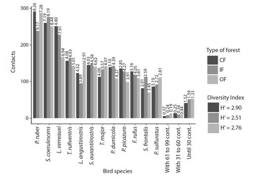
Fig. 7 Most abundant species in the levee forest physiognomies. The relative abundance (Pi) value for each species is shown on the bars.
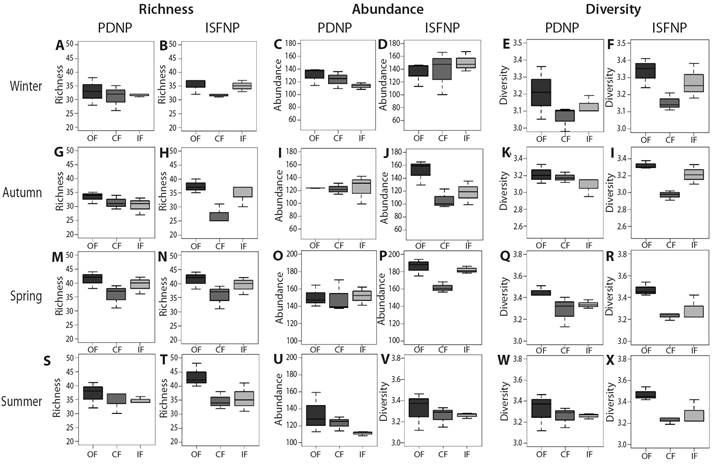
Fig. 8 Bird differences of richness, abundance and diversity among forest types in each season, in each park. A. Winter richness in PDNP. B. Winter richness in ISFNP. C. Winter abundance in PDNP. D. Winter abundance in ISFNP. E. Winter diversity in PDNP. F. Winter diversity in ISFNP. G. Autumn richness in PDNP. H. Autumn richness in ISFNP. I. Autumn abundance in PDNP. J. Autumn abundance in ISFNP. K. Autumn diversity in PDNP. L. Autumn diversity in ISFNP. M. Spring richness in PDNP. N. Spring richness in ISFNP. O. Spring abundance in PDNP. P. Spring abundance in ISFNP. Q. Spring diversity in PDNP. R. Spring diversity in ISFNP. S. Summer richness in PDNP. T. Summer richness in ISFNP. U. Summer abundance in PDNP. V. Summer abundance in ISFNP. W. Summer diversity in PDNP. X. Summer diversity in ISFNP.
Bird diversity varied among forest types in all the seasons. In winter, 56.76 % of bird diversity variation was explained by an additive model including forests and sites (AICc = -26.6, w = 0.67), with differences between OF and CF types (P < 0.01), with OF being more diverse than CF. Regarding sites, ISFNP was more diverse than PDNP (P < 0.05). In autumn, the greatest diversity occurred in CF of PDNP (P = 0.004). In spring, the additive model of forests and sites explained 63.08 % of the variation (AICc = -28.10, w = 0.78), with diversity being highest in OF, intermediate in IF, and
lowest in CF (P < 0.05). According to the differences between sites, the ISFNP was the most diverse (P < 0.05). In summer, CF were the least diverse (P < 0.01) (Table 2, Table 3, Fig. 7, Fig. 8).
Discussion
Differences in vegetation structures (tree cover, shrub cover, herbaceous cover, and height) were found to be related to forest types mainly. The maximum shrub cover was recorded in Intermediate Forests (IF) and herb cover in Open Forests (OF) might be due to the greater light availability at the lower vegetation levels, reaching the lower forest strata due to the open canopy structure. OF might be considered edge environments favored by abiotic factors, especially light, which generates microclimatic variations that increase plant diversity (Granados-Sánchez et al., 2006; Nieves-Vele & Orellana-Peralta, 2018); in turn, these conditions are considered optimal for bird diversity (Baker et al., 2002; Rannestad et al., 2015). It is known that the development of the different vertical vegetation strata is enhanced when a disturbance of the forest canopy increases light availability (Anderson et al., 1978), with solar radiation being a factor determining the natural regeneration of forest vegetation (Viana & Jardim, 2013). In closed canopy forests, most of the light is absorbed by the tree canopy, reducing the development of the understory vegetation.
Our records of birds for the Delta wetland area were like those previously reported (eBird, 2020; Frutos et al., 2020a; Frutos et al., 2020b; Magnano et al., 2019; Ronchi-Virgolini et al., 2011; Rossetti & Giraudo, 2003). Overall, our results show that closed forests (CF) had the lowest richness, abundance and diversity values in their bird communities, whereas the highest values of richness, abundance and diversity were detected in OF. In a highly heterogeneous environment, niche availability is high; therefore, species richness is high while evenness is low, reducing diversity (Rosenzweig, 1995; Symonds & Johnson, 2008). Other authors argue that a greater niche availability drives greater evenness (Cotgreave & Harvey, 1994). However, community structure depends on landscape structure and spatial scale (Drobner et al., 1998; Horlent et al., 2003). Based on the results of our analyses of forest types and birds, we could suggest that a more heterogenous ambient could host more diversity, regardless of the bird community evenness. The richness record observed in the OF zone exemplifies this phenomenon, where the environmental heterogeneity manifests through variations in the vegetation strata. Similar results have been reported for the extensive floodplain of El Kilombero in Tanzania, a prominent wetland in East Africa (Rannestad et al., 2015). Further investigations emphasize the pivotal role played by edge habitats (Baker et al., 2002; Miller et al., 2004) in structuring avian communities. Considering that the levees of the OF zone host the most diverse avian communities and are near water, it is plausible to suggest that they function as well as exhibit characteristics emblematic of edge environments.
PD National Park has held protected status for several decades, while ISF National Park attained protection approximately a decade ago, resulting in the recent cessation of livestock farming activities (Frutos et al., 2018). Given the disturbing effects of recent livestock farming, it was expected that ISFNP would present some difference with respect to PDNP in terms of the lower vegetation strata, as suggested by Olff & Ritchie (1998) and Frutos (2018) as an effect associated with the intermediate disturbance hypothesis. Our findings show no differences in vegetation strata among the study sites, despite their different management histories. Nevertheless, the avian variation pattern proved to be non-uniform, which could be attributable to the influence of the characteristics of the area and seasonal fluctuations in vegetation. The recent cessation of livestock activities in ISFNP may have contributed to the proliferation of shrubs, resulting in subtly elevated coverage values at this location. Despite the increase in the prevalence of shrubs, typically correlated with higher avian diversity (Godoi et al., 2017; Martin, 1993), this trend was not conspicuously apparent. Considering potential seasonal disparities linked to abiotic/climatic factors in the coverage of lower strata (Zerda & Tiedemann, 2010), we could attribute the differences in the presence or absence of certain species in the parks. Examples include Phacellodomus striaticollis (insectivore of the shrub stratum), Asthenes pyrrholeuca (migratory insectivore of the shrub stratum), Saltator similis (fruit-insectivore of the low canopy), and Patagioenas maculosa (terrestrial granivore), all of which were notably absent in PNPD. This absence could be correlated with reduced habitat diversity in the understory and soil strata. This phenomenon could be correlated with an increased herbaceous vegetation density in the early stages of plant succession, a result of the absence of herbivory, particularly by livestock. In contrast, this form of herbivorous activity was prevalent in ISFNP in the past but has been systematically excluded from the site since its official designation as a national park, slightly over a decade ago. This exclusion creates more open space in the lower vegetation strata, potentially enhancing resource availability and eliciting corresponding avian responses to intermediate disturbance states in the environments (Frutos et al., 2018). In this context, the absence of Myiothlypis leucoblephara (insectivore inhabiting shrubbery and soil strata) in ISFNP can also be ascribed to a scenario favoring the occupation of other dominant species in the soil stratum, resulting in displacements of less dominant species within the assemblage. Additional species such as Limnoctites sulphuriferus, Aramus guarauna, and Aramides ypecaha (species associated with salt marshes) were absent in PDNP (yet present in ISFNP), potentially linked to the lower prevalence of salt marshes near the sampling points in this park. These absences are not of particular concern, as these species do not hold emblematic status for the region. According to the International Union for Conservation of Nature [IUCN] (2023), none of the species is classified as threatened, vulnerable, or endangered globally; instead, all are categorized as least concern. This aligns with the regional survey conducted by specialists from Aves Argentinas (2015).
However, we found differences in the arrangement of birds associated with parks, in terms of richness, abundance and diversity, with seasonal influence. This result suggests that despite past anthropogenic activities in the study sites, spatial heterogeneity of the forests in the floodplains is still high, possibly due to the dynamics contributed by the pulses. Thus, taking into account that the significance of the analysis that compared vegetation strata between sites was very close to the acceptance limit, it could be considered that the natural history of parks associated with livestock in natural riparian environments in some cases favor bird diversity (Frutos et al., 2020a; Frutos et al., 2020b; García et al., 2008; Martin & Mcintyre, 2007), however, it is not a necessary requirement to maintain a heterogeneous and beneficial structure for the dynamics of birds in riverine environments. Vegetation in the islands reveals ecological processes with several successional stages, caused by regimes of seasonal hydrological disturbances (Aceñolaza et al., 2005; Malvárez, 1999). Therefore, river wetlands are highly heterogeneous and maintain a high array of small habitats and microhabitats (Miller et al., 2004; Tavares et al., 2015).
The distinct resource offerings determined by the floristic composition in each type of forests and in each park were not analyzed to observe seasonal changes in that aspect. However, the analysis of vegetation cover in each forests type revealed variations throughout the seasons, particularly in the herbaceous layer (in terms of both coverage and height of the plants). Regarding the seasonal variation detected in the bird community, we can highlight that OF were not consistently able to distinguish themselves with a higher richness value in all seasons. Nevertheless, during the summer, lower abundance values were evident in the interior forests. Conversely, in autumn, there was a notable increase, particularly in PNPD. In CF, we found the lowest bird abundance value in autumn, and in general, the lowest value of diversity across seasons. There may be a relationship among the type of resources offered by the CF, a decrease of those resources in cool seasons and preferences for these resources by the species present there. To explain this relationship, a species composition analysis might be necessary to detect species preferences for different physiognomies (Horlent et al., 2003). We speculate, based on our results, about the existence of a dynamism that is not easy to identify in the arrangement of the community. This dynamism appears to be generated by the combination of seasonal and microspatial factors.
According to the classical niche theory, different species are associated with different habitat types; therefore, a few small and overlapping habitats may hold a high number of species (Allouche et al., 2012; Laanisto et al., 2013; MacArthur & MacArthur, 1961). Environmental heterogeneity is the degree of variation of the landscape components (physiognomy, structure, size, relative spatial arrangement) both at the spatial (different successional stages) and temporal levels (relationship between flooded areas and emergent areas in floodplains). It acts as a stabilizing mechanism that smooths the shift from stable to alternative states (van Nes & Scheffer, 2005) and determines the degree of habitat suitability for wild species, conditioning their richness, abundance and permanence in the area (Bó & Malvárez, 1999; Bó et al., 2010, Robinson et al., 2002). Therefore, environmental heterogeneity is a more important predictor of spatial variation of bird richness than the area covered by each habitat type (Lorenzón et al., 2016).
Beta diversity and species turnover from one area to another have a substantial influence on general species richness in a region (Ronchi-Virgolini et al., 2011; Vellend, 2001). The variation of the assemblage between sites, independently of the variation contributed by the physiognomies of the forests, could be related to the floristic composition. This variation would provide specific perches, shelters, or feeding sites for the birds and influence the decision to choose one site over another. But the seasonal differences in bird assemblage between sites also might be influenced by the migratory effect. Seasonal variations in the bird assemblages, caused by migrations, have been widely studied (Capllonch et al., 2008; Capllonch, 2018; Carvalho et al., 2013; Lima et al, 2021). The studied wetlands are in the fluvial biological corridor of the Paraná River. The relative position of the national parks studied in the great corridor and their proximity to migratory routes might be additional variables that influence the preference for one site or another and, therefore, in the arrangement of bird communities between sites.
In bird assemblages of highly heterogeneous riparian environments, seasonal changes are very evident (Lima et al, 2021; Lorenzón et al., 2019; Ronchi-Virgolini et al., 2013), which may explain the high seasonal variation of our results, regardless of microspatial variation. However, it should be noted that the migratory condition would not allow us to predict habitat selection (Horlent et al., 2003); therefore, the effect of migration on forests preference would rather be random.
The variation detected within levee forests shows that a deeper analysis is needed for differences in composition among vertical strata of the understory (De Stefano et al., 2012). Thus, the differential niche offer that optimizes resources for birds could be more clearly evidenced, considering that the turnover rate in plant composition is high in these environments. Therefore, deeper analyses of the differences in the bird assemblage using a functional classification criterion, i.e., guild, may reveal subtle aspects that are poorly detectable from a general perspective (Farías et al., 2007; Milesi et al., 2002; Ronchi-Virgolini et al., 2011; Root, 1967). Guild-based analyses would contribute more specific information to properly guide conservation efforts in these wetland environments, where variation at different scales is clear.
We conclude that there are at least three categories of levee forests on floodplains determined by differences in their vegetation cover, and that birds respond differentially to these conditions. These findings show the importance of habitat heterogeneity in river-associated island environments and highlight the importance of the microhabitat scale in the levees of floodplains. This allows us to focus on the underlying dynamics at this scale and understand the changes that occur in line with the evolutionary histories of the sites, and the recovery of environments, while also considering the changes associated with seasonal cycles. It is evident to us that, within these wetland landscapes, emphasis should not solely be placed on the mosaic at a macro scale. It is crucial to concentrate on microspatial dynamics to gain a more profound understanding of the concealed biological processes within the islands of these tropical and subtropical environments, where heterogeneity is apparent. We believe that considering the micro-scale environmental heterogeneity of levee forests in riparian environments is an important strategy for planning wetland conservation management. This study, in addition to evidencing and highlighting the existence of differential microhabitats within the levee forests, reflects upon the vegetation dynamics, bird behavior and the transition of the riparian forest in its recovering towards a more natural state, where the pulse of the river and the effect of seasonality do not stop operating.
Ethical statement: the authors declare that they all agree with this publication and made significant contributions; that there is no conflict of interest of any kind; and that we followed all pertinent ethical and legal procedures and requirements. All financial sources are fully and clearly stated in the acknowledgments section. A signed document has been filed in the journal archives.

