


 English (pdf)
 Article in xml format
 Article references
 Send this article by e-mail
 Cited by SciELO
  Similars in
SciELO
Similars in
SciELO  uBio
uBio 
 Permalink
Introduction
Pelagic fishes such as the common dolphinfish (Coryphaena hippurus L) are highly migratory in tropical and subtropical waters (Zúñiga-Flores, 2009). However, similarly to other species, their mobility is restricted by oceanographic variability, which determines their survival, growth, and development (Bellido et al., 2008; Blaxter & Hunter, 1982). Generally, changes in environmental conditions trigger fish migration, which can last for several months across big areas, generating good conditions for fishing (Bellido et al., 2008).
Several studies have indicated that the environmental variables in oceans influence the distribution of pelagic fish species such as the dolphinfish (Hsu et al., 2021). The physiology of this species restricts populations to occur in areas where the sea surface temperature (SST) varies between 21.5 °C and 27.5 °C, and chlorophyll-a (Chl-a) between 0.01 mg/m3 and 9.5 mg/m3 (Guzmán et al., 2010). It has been demonstrated that SST is an accurate predictor of habitat distribution, because it holds a close relationship with species richness and plays a vital role in the physiology of pelagic fish. On the other hand, Chl-a is recognized as an important oceanographic parameter as it determines primary production and biological productivity in oceans. Several findings suggest that SST and Chl-a are key factors influencing patterns of spatial distribution and abundance variability of pelagic fish like tuna, swordfish, and the common dolphinfish. However, for this last species, the spatial distribution of potential fishing zones (PFZ) in the tropical region (particularly in the Colombian Pacific Ocean), and their controlling factors are not clear enough (Zainuddin et al., 2013).
A PFZ is a prediction of fish aggregation in specific areas across the ocean, which is made based on the relationship of fish biology and the environmental context. PFZs are generally made using statistical parameters of SST and Chl-a (Natteshan & Kumar, 2016). Different researchers have applied and discussed a wide range of techniques for the prediction of PFZs, including remote sensing of a variety of oceanographic variables, geographic information systems (GIS) and statistical approaches such as Generalized Linear Models (GLM), Generalized Additive Models (GAM) and Classification and Regression Trees (CART). These approaches ultimately find the functional links between the environmental information and fish abundance data to produce a PFZ prediction (Marín-Enríquez et al., 2018).
Research published by Salvadeo et al. (2020) and Marín-Enríquez et al. (2018) show the application of these techniques to identify the distribution of dolphinfish along Southern California and the Mexican coast Herrera-Montiel et al. (2019) adopted this approach to identify and evaluate the PFZs of seerfish (Scomberomorus sierra) in the CPO. The identification of PFZs has several challenges associated with the requirements of habitat modeling, because, beyond the relationship between fish abundance and their environment, other factors such as management, the spatiotemporal variation of population sizes, the existence of regulatory zones for fishing and the damage to marine ecosystems have also an influence on fish distribution (Selvaraj et al., 2009).
Colombia is a country where fisheries contribute significantly to the economic growth and food security (FAO, 2021), hence the application of habitat models to determine patterns of abundance, spatial distribution, and the relationship of these patterns with the characteristics of the habitat and the fishing areas, is of crucial importance (Salazar et al., 2021; Selvaraj et al., 2009). Furthermore, considering the rapid changes of fish populations due to climate change in the oceans, it is highly important to determine their PFZs, specially for commercial fishes such as C. hippurus. So far, there is no yet available information on this issue.
Consequently, this research aimed at building, running, and comparing different models to predict the PFZs of C. hippurus in the CPO, considering the influence of determinant environment conditions for the species suitability.
Materials and methods
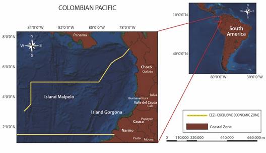
Study area: The CPO belongs to the Eastern Pacific Ocean, which is located along the West coast of Colombia. It has a coast length of 1 300 km and borders to the North with the isthmus of Panama and to the South with Ecuador (Fig. 1). The oceanographic conditions of CPO are subject to the seasonal changes in the position of the Inter-Tropical Convergence Zone (ITCZ) and to the strong inter-annual changes due to El Niño South Oscillation (ENSO), both irregular fluctuations that involve changes in the general circulation of winds, insolation and hydrography across the Tropical Eastern Pacific (Rodríguez-Rubio et al., 2003). ENSO implies an unstable interaction between the SST and the atmospheric pressure, causing strong variability in the winds, precipitation and the depth of the thermocline, affecting the biological productivity and the reproduction and survival of marine species (Beltrán, 2011; Fiedler, 2002) (Fig. 1).
Data sources and structure: Catch data of C. hippurus was provided by the fishery Sepulveda Rodgers LTDA and contains the historical catch data of semi-industrial fishing boats in the study area during the species’s season (November to March), from years 2000 to 2010, 2012 and 2015. These catches were performed with longlines of 1 100 circular hooks. The number of captured fish divided by the 1 100 total hooks is reported here as the Catch per Unit of Effort (Selvaraj, 2010), which is a proportion ranging from 0 to 1. Each CPUE value results from a particular fishing set, from fishing trips that last between 2 and 10 days at the sea. Each particular CPUE value represents the catch efficiency, and indirectly, the fish abundance during each of the 150 total fishing that occurred during the studied period. All the CPUE values were positive, implying no zero catches. Additionally, each CPUE is linked to a geographical position where each fish trip was performed along the 800 km of the CPO.
Oceanographic variables: Satellite data of SST and Chl-a was obtained from the MODIS sensor (Moderate Resolution Imaging Spectroradiometer) at the website http://www.oceancolor.gsfc.nasa.gov/. We downloaded daily L3 level data (4 km) that matched the catch dates for the period 2002-2015. Data of Sea Level Anomalies (SLA) was obtained from the AVISO project (Archiving Validation and Interpretation of Satellite Oceanographic data), which is supported by the Centre National D’Etudes Spatiales (CNES) in France (Piedrahíta et al., 2013) (http://www.las.aviso.oceanobs.com/las/getUI.do). SLA data was combined to available information from satellites ENVISAT, ERS1/2, GFO, JASON1, JASON 2 and TOPEX/POSEIDON, with a spatial resolution of 0.25 decimal degrees. The bathymetric information was acquired from the website: https://www.ngdc.noaa.gov/mgg/global/ with a spatial resolution of 1 minute of arc (1 km). This resolution was modified to 4 km by using a bilinear resampling algorithm in ArcGIS version 10.5. This oceanographic data set was processed together with the fishing data in order to build the models for PFZ’s prediction of C. hippurus in the CPO (Table 1).
Table 1 Data sets used to build the predictive statistical models and their sources.
| Data sets | Source | Period | Spatial Reference | Resolution | |
| Spatial | Temporal | ||||
| C. hippurus captures | Records from Sepúlveda Rodger Ltda | 2000-2010 2012 and 2015 | GCS_WGS_1984 | NA | Daily |
| Chl-a | MODIS sensor | 2002-2015 | GCS_WGS_1984 | 4 km | Daily |
| TSM | MODIS sensor | 2002-2015 | GCS_WGS_1984 | 4 km | Daily |
| SLA | ENVISAT, ERS1/2, GFO, JASON1, JASON 2 y TOPEX/POSEIDON | 2002-2015 | ITRF2008 | 4 km | Daily |
| Bathymetry | ETOPE 1 | 2002-2015 | GCS_WGS_1984 | 1 km | NA |
Statistical modeling: The prediction of the spatial distribution of PFZ’s of C. hippurus was performed using parametric and semi-parametric statistical models such as GLMs and GAMs respectively. GLMs were used as they allow the use of specific probability distributions appropriate for normal errors (Gaussian), asymmetric errors (Gamma) and errors coming from proportion data (Beta); plus, link functions to account for nonlinear relationships between predictors and responses (Myers et al., 2012). GAMs were used because besides specifying specific probability distributions and link functions, they offer the flexibility of fitting nonlinear relationships via smoothed functions (spline or kernel) combined with parametric functions. Both models perform parameter estimation via Maximum Likelihood Estimation (MLE), (Wood, 2017).
GAM:

Where g is a link function, µ i is the expected value of the response variable (CPUE), a0 is a model constant for every oceanographic predictor, S n is a smoothing function for each predictor and e is a random error (Wood, 2017) with a specific probability distribution (Table 2).
Table 2 Results of the modeling and validation procedures showing the type of model, probability distribution of errors, link-functions and the metrics used for model selection and validation.
| Modeling | Validation | ||||||
| Model | Probability distribution | Link-function | Df | AICc | Adjusted R2 | D | RMSE |
| GAM | Gaussian | Log | 14 | -525.5 | 0.50 | 54.2 % | 0.037 |
| GAM | Gamma | Log | 10 | -526.2 | 0.38 | 34.9 % | 0.040 |
| GAM | Beta | Logit | 10 | -522.4 | 0.39 | 41.1 % | 0.040 |
| GLM | Beta | Logit | 4 | -525.4 | 0.28 | 25.2 % | 0.044 |
| GLM | Gaussian | Log | 6 | -494.2 | 0.27 | 30.1 % | 0.045 |
| GLM | Gamma | Log | 6 | -519.3 | 0.17 | 27.4 % | 0.052 |
Df = degrees of freedom.
GLM:

Where is a link function, Yi is the ith observation of CPUE, X 1i , X 2i , X ki are the ith observations of the k oceanographic predictors, µ i is the ith term of the random error with a specific probability distribution and b1, b2 b k are the effect parameters for each predictor (Espinoza-Morriberón, 2010).
These models were built with all the oceanographic variables as predictors using a random data subset with 70 % of the dataset (N = 105). The remaining 30 % (N = 45) was kept for model validation (see next section). The Akaike Information Criterion (AIC) (Akaike, 1973; García et al., 2014), the coefficient of determination (R2) and the explained deviance (D) were used as the criteria to select the best model among all candidate models that were built. To identify differences in CPUE between months of the year, we used a Kruskal-Wallis test plus a-posteriori pairwise multiple comparisons (Zar, 2010), where P values lower than 0.05 were considered as statistically significant.
To identify spatial and temporal autocorrelation patterns in the CPUE data that would risk the reliability of the model predictions, we performed Moran tests (Legendre, 1993) and Partial Autocorrelation Functions (PACF) (Tsitsika et al., 2007) respectively on the residuals of the best model selected after model validation. Moran test showed no significant spatial autocorrelation between residual values and the matrix of spatial distances (P = 0.69) between catch points, and the PACF showed only a weak autocorrelation in lag 1 (R = 0.22). For Gaussian GAM and GLM models, normal distribution and homoscedasticity were checked by performing QQ-plots and residuals vs fitted plots. All these assumptions were correctly fulfilled to ensure model validation and applicability for PFZs prediction.
Model validation: We used a cross-validation approach for the predictions of CPUE (Pérez-Planells et al., 2015). This approach was performed with a random subset containing 30 % of the data that was not involved in modeling. We used the Root Mean Square Error (RMSE) as a metric to evaluate prediction accuracy validate and model performance. This metric quantifies the quality of predictions through the difference between the observed and predicted values (Martínez, 2016). RMSE is calculated as:
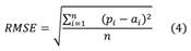
Where is the actual observed value, is the predicted value and is the number of observations. All the statistical analyses were performed in R-studio (ver 1.1.442) with packages base, MuMin, ggplot2, mgcv, ape, metrics, betareg, boot and raster.
Results
Oceanographic variables: SST varied between 25.13 and 29.06 ºC, being higher in January and lower in March. Higher values of CPUE occurred in temperatures between 25.5 and 27.5 ºC. Above 27.5 °C and below 25.5 °C, CPUE decreases. Chl-a varied between 0.15 and 2.2 mg/m3, being higher in December and February. Higher values of CPUE occurred in places where Chl-a varied between 0.5 and 2.2 mg/m3, Below and above these values respectively, CPUE decreased. SLA varied between -21.18 and 8.9 cm. Higher CPUE values occurred between -10 and 0.1 cm. Below and above these values respectively, CPUE decreased. Bathymetry varied between -24 and -400 m, with no optimal ranks for CPUE.
Model selection and validation: According to the values shown in Table 2, the Gaussian GAM, Beta GAM, and Gamma GAM were the best candidate models. Despite Gamma GAM had the lowest AICc (slightly lower than the Gaussian GAM), the R2 and D values were considerably higher for the Gaussian GAM. Similarly, the RMSE values for the cross-validation procedure showed that the predictions resulting from Gaussian GAM were the best fitted to the observed CPUE data. When plotting CPUE predictions over the years (Fig. 2A), Gaussian GAM was able to capture higher time variability than other models. This was particularly conspicuous over periods of abrupt oscillations in fish captures like those between 2001-2003, 2006-2009 and 2010-2015. When comparing the CPUE predictions of every model to the observed CPUE (Fig. 2B) and fitting simple linear regressions on the data, we found again a higher performance for Gaussian GAM, which had a higher slope (0.7) and lower intercept (0.03) in comparison to Gamma GAM and Beta GAM.
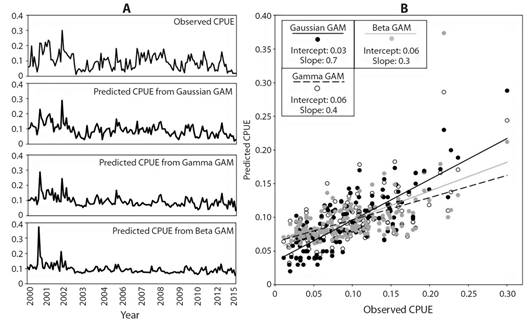
Fig. 2 A. Total observed and predicted CPUE values over capture years for the whole study area according to the three best candidate models: Gaussian GAM, Gamma GAM, and Beta GAM. Predictions are shown in the original CPUE scale after exponential transformation of fitted values. B. Relationship between observed and predicted CPUE values according to the three best candidate models. Lines represent a linear regression between the observed and predicted CPUE data for every model. Intercept and slope parameters are shown in the upper boxes for every model.
Despite all these criteria in favor of Gaussian GAM, it is clear that this model still underestimates CPUE and its R2 cannot be considered high. However, due to the high variability of these kinds of data both in the spatial and temporal dimensions and to the multiplicity of factors not able to be included in our models, we considered that the performance of Gaussian GAM was enough as a first approach to the prediction of PFZ’s for C. hippurus in the CPO. The results of the Gaussian GAM are shown in Table 3. For this model, the intercept as well as the effect of Chl-a, SST, and SLA were statistically significant, yet based on the F-values, Chl-a had the highest effect on the behavior of CPUE.
Table 3 Parametric coefficients and approximate significance smooth terms resulted from Gaussian GAM model.
| Parametric coefficients | ||||
| Estimate | SE | t-value | P-value | |
| Intercept | 0.08 | 0.04 | -59.45 | < 0.001 |
| Approximate significance of smooth terms | ||||
| EDF | RDF | F-value | P-value | |
| Chl-a | 2.84 | 3.47 | 17.56 | < 0.001 |
| SST | 4.86 | 5.60 | 2.08 | 0.05 |
| SLA | 3.50 | 4.28 | 3.62 | 0.006 |
| Bathymetry | 1.00 | 1.00 | 0.01 | 0.91 |
EDF = Effective degrees of freedom; SE = Standard error; RDF = Reference degrees of freedom.
Prediction of PFZs: Using the CPUE predictions of the Gaussian GAM, we generated a series of maps according to the monthly seasonality of C. hippurus (November-March) for all the capture years (2002-2015) (Fig. 3). These maps show the probability of aggregation of C. hippurus, and consequently, reflect the occurrence of PFZs across the CPO. The spatial distribution of PFZs during November expanded uniformly from coordinates 1°00’ N & 79°00’ W to 8°00’ N & 83°00’ W along the Pacific coast of Colombia. Meanwhile, the PFZ’s distribution in the oceanic area was not uniform in comparison to the coast. However, important fish aggregation was observed between coordinates 6°00’ N & 80°00’ W (coastal area) and 4°00’ N & 82°00’ W (oceanic area), especially to the South (border with Ecuador) in the Nariño region, with CPUE values around 0.24. In December, the PFZs are mainly grouped in front of the Nariño region, similarly to the pattern of November, with CPUE values ranging from 0.17 to 0.19 between coordinates 6°00’ N & 77°05’ W to 1°00’ N & 79°05’ W near to the coast. Two oceanic conglomerations were observed at coordinates 3°00’ N & 81°02’ W to 2°00’N & 82°00’ W and 2°08’ N & 82°03’ W to 1°05’ N & 82°03’ W approximately. Mean CPUE values of December are lower in comparison to November, with maximum values up to 0.234.
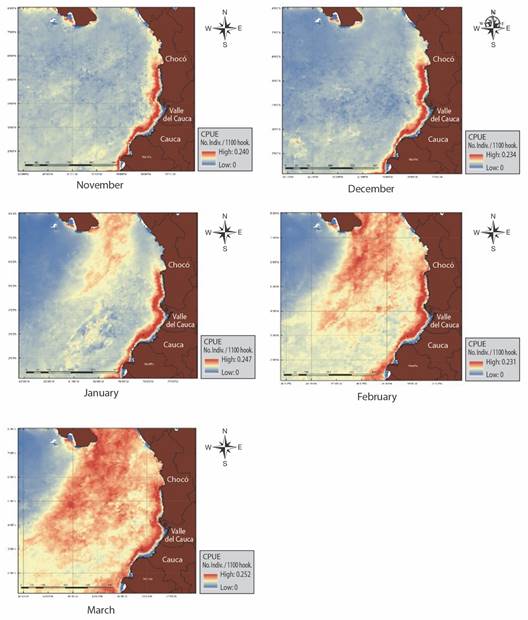
Fig. 3 Assemble maps of monthly predicted PFZs for C. hippurus during 2002 to 2015 in the Colombian Pacific Ocean.
For January, PFZs show a persistent occurrence in front of the Colombian coast from coordinates 6°00’ N & 77°05’ W to 8°00’ N & 78°5’W to 1°00’ N & 83°1’ W, with mean CPUE values around 0.24. This zone starts on the Panama coast and extends southwards to the Chocó and Valle del Cauca regions in the Colombian coast, with a mean CPUE of 0.24, which gradually decreases towards the Cauca and Nariño regions. CPUE values in January were significantly higher than in December and November for all the study years. During February there were two conspicuous PZFs, one between coordinates 1°17’ N & 79°00’ W to 6°53’ N & 77°42’ W and the other at the oceanic area of the Panama basin from coordinates 7°18’5’’ N & 79°46’ W to 3°20°N & 80°83’ W. Mean CPUE values in these zones are around 0.18.
Finally, the spatial distribution of PFZs for March showed higher CPUE values. Locations of PFZs persisted near the coast at coordinates 6°00’ N & 77°5’ W to 1°00’ N & 79°05’ W and at an oceanic area with coordinates 3°00’ N & 81°02’ W to 2°00’ N & 82°00’ W, 2°08’ N & 82°03’ W and 1°05’ N & 82°03’ W approximately. Generally, the PFZs were spatially persistent over the months and years. Nevertheless, the PFZs with larger sizes occurred during January, February, and March, with mean CPUE values around 0.25. The difference of CPUE values between all pairs of months were highly significant according to Kruskal-Wallis tests (P < 0.001 for every a-posteriori pairwise multiple comparison).
Discussion
The GIS approach used in this study was successful to capture enough variability in the oceanographic variables, which helped to understand the spatiotemporal dynamics of the PFZs of C. hippurus. This is in accordance with the results described by Devis et al. (2002), where the variation in Intertropical Convergence Zone (ITCZ) triggers changes in SST and Chl-a. This phenomenon creates a gradual seasonality in climate and oceanic conditions, allowing the presence of different temperatures along the surface water. Concerning the spatial distribution of SST, our results resemble the findings of Rodríguez-Rubio (2003), who mentioned that this variable evolves seasonally between January and March, when surface waters of low temperature (25-26 °C) extend from the Gulf of Panama to the center of the basin in a South-to-Southwest orientation. From April to June the temperature increases gradually eastwards and by July-September, the cold-water plume disappears altogether with 3 °C increase to the North and 1 °C decrease to the South. By the end of the year (October-December), the spatial pattern of temperature stays, though with a ~1 °C decrease in across the CPO.
On the other hand, the results obtained with the GAM model with Gaussian distribution are in accordance with the findings made by Bigelow et al. (1999), Rodríguez-Marín et al. (2003), Zagaglia et al. (2004), Zainuddin et al. (2013), and Setiawati et al. (2015). These authors indicated that this modeling approach is highly efficient to predict PFZs of pelagic species in the Pacific and Atlantic oceans. This efficiency relies on the fact that GAMs offer high flexibility regarding the type of data and the link between predictors and responses, allowing non-linear and non-monotonous relationships to make predictions in the response variable (França & Cabral, 2015; Guisan et al., 2002; Yee & Mitchell, 1991). Maunder and Punt (2004), compared the performance of GAMs, GLMs and GLMMs (Generalized Linear Mixed Model) to predict the spatial distribution of valuable fish species such as tuna and sharks, remarking the benefits of GAMs.
Though we consider that the Gaussian GAM model used in this study was successful as a first approach to predict the spatial distribution and PFZs of C. hippurus in the CPO, our results suggest that the precision of the model still needs to be increased for better results. When observing the model predictions over the capture years in (Fig. 3), it is clear that for many capture months the model underestimates or overestimates the observed CPUE, with maximum difference values up to 9.6 %. We suggest that these underperformances can be solved by including other biological variables not considered in this study, such as physiologic traits, life-history traits, genetic structuring, predation, and migration rates of C. hippurus populations. When including some of these variables in the model, a higher CPUE variability could be captured, hence increasing the chance of making more accurate predictions. This would help the developing of more powerful frameworks for studies that consider fish management and decision making under climate change scenarios.
Our model detected Chl-a as the most efficient to predict CPUE, agreeing with Sund et al. (1981), who considers it as the most restrictive oceanic variable for the horizontal and vertical distribution of pelagic species. Furthermore, it has been a successful proxy to estimate the available food in pelagic ecosystems, since this pigment is present in most of the phytoplankton species and forms the basis of trophic chains (Martínez-Rincón, 2012; Sartimbul et al., 2010). Loukos et al. (2003) suggested specific large-scale changes on the fish habitat in the equatorial Pacific by means of SST effects, which could explain the distribution of available habitats for pelagic fishes on higher latitudes due to the increase of temperature by global warming (Cheung et al., 2009; Mugo et al., 2010). Despite SLA and Bathymetry showed a lower effect on the CPUE, they were included in the model because they are related to the spatial distribution and movement of pelagic species (Maravelias, 1999). SLA is related to mesoscale cyclonic movements that occur at the beginning of the year (Rodríguez-Rubio, 2003), bringing oceanic upwelling, low temperatures, and high chlorophyll concentrations. According to Sabarros et al. (2009), it is highly probable that these mesoscale processes are related to the presence of PFZs of pelagic fishes.
The predicted PFZs for C. hippurus and their spatial distribution was similar to the findings drawn by Lasso and Zapata (1999), who mentioned that the higher fish abundances occur during February and March. Furthermore, this season could be associated with phenomena that trigger fish migration, since it coincides with the lowest SST and higher Chl-a concentrations in comparison to the rest of the year. Giraldo et al. (2010) and Guzmán et al. (2010) demonstrated that the aggregation of C. hippurus are linked to mesoscale oceanic processes, such as the oceanic thermal fronts. Lasso and Zapata (1999) suggested that the migratory path of C. hippurus could be associated with surface ocean currents in the eastern Pacific, as a response to the changes driven by ENSO, which cause fish populations to migrate southwards in search for warmer waters (Caetano-Nunes, 2013; Lasso & Zapata, 1999).
The predicted PFZs shown by our model from February and March agree with the reports of the highest catch rates in Colombia (Lasso & Zapata, 1999) an also, with the isotherm changes from January to April, and the salinity increase in the Pacific Ocean that brings an upsurge of nutrients in front of the Panama Bay (Valencia et al., 2013). Generally, these results show that the distribution patterns of PFZs for C. hippurus are associated with changes in SST, which influence fish aggregation, growth, reproduction, and survival (Boyce et al., 2008; Martínez-Rincón, 2012).
As shown in this study, the identification of PFZs of fish species emerges from the combination of remote sensing, geographic information systems, historical registers of in situ data and statistical modeling tools, which can be used as a robust package to improve the management and decision making of fish resources. As stated by Selvaraj et al. (2009), the maps resulting from this multidisciplinary approach can be used for conservation o extraction purposes. However, to achieve these purposes, we still need a standardization of data sharing, data depuration and analysis and training of the entities and people in charge of its administration and distribution.
The development of these prediction techniques has created new alternatives that allow understanding the behavior and distribution of fish populations. However, the variability of the prediction performances among different models results in contrasting predictions. This implies that a predictive model must be selected very carefully, especially if it is intended for practical applications (Zhang et al., 2017). The advantage of using GAMs relies to their robustness to outliers and its ability to capture complex interactions between predictors. These advances in the model’s predictive power allow a more reliable understanding of potential fishing areas, especially in those areas at the local level (Venables & Dichmont, 2004).
Ethical statement: the authors declare that they all agree with this publication and made significant contributions; that there is no conflict of interest of any kind; and that we followed all pertinent ethical and legal procedures and requirements. All financial sources are fully and clearly stated in the acknowledgements section. A signed document has been filed in the journal archives.

