


Services on Demand
Journal
Article
 English (pdf)
 Article in xml format
 Article references
 Send this article by e-mail
Indicators
-
 Cited by SciELO
 -
 Access statistics
Related links
-
 Similars in
SciELO
Similars in
SciELO  uBio
uBio
Share

 Permalink
Revista de Biología Tropical
On-line version ISSN 0034-7744Print version ISSN 0034-7744
Rev. biol. trop vol.54 n.2 San José Jun. 2006
Distribution and habitat suitability index model for the Andean catfish Astroblepus ubidiai (Pisces: Siluriformes) in Ecuador
Luis A. Vélez-Espino
Environmental and Resource Studies Program, Trent University, Peterborough, Ontario, K9J 7B8, Canada. Fax: 1(705) 748-1026; 1(705) 748-1569; tonovelez@yahoo.com Current address: 70 Chesterton Lane. Guelph, Ontario, N1E 7A6. Tel. (519) 780-1681.
Received 03-III-2003. Corrected 19-XII-2003. Accepted 12-III-2004.
Abstract. In conservation biology there is a basic need to determine habitat suitability and availability. Astroblepus ubidiai (Siluriforms), the only native fish in the highlands of Imbabura province in the Ecuadorian Andes, was abundant in the past in the Imbakucha watershed and adjacent drainages, but currently it is restricted to a few isolated refuges. Conservation actions are needed if this unique fish is to persist. A Habitat Suitability Index (HSI) for the species has been developed in order to aid management decisions. In this HIS model biomass density (B) was selected as a better indicator of habitat quality than either abundance or density. A population well-being index (PI) was constructed with the combination of B and an indicator of fish health (proportion of fish in the population with parasites and deformities). Based in other models of benthic fish the habitat variables current velocity, flow, depth, width, cover, invertebrate composition, vegetation type, terrestrial vegetation, land use, substrate, temperature, pH, TDS, oxygen, altitude, and slope were included in the analysis. An anthropogenic perturbation index (H) and a fragment isolation index (FII) were developed and included as habitat variables as well. The HSI model was applied to refuges and a sample of 15 aquatic bodies without fish populations within the study region. From the sampled sites without A. ubidiai 26.6% presented low quality, and the remaining 73.3% had medium quality according to the HSI estimated. Good quality habitat for dispersal, escape or translocations is rare in the region. The low HSIs estimated in some of the refuges suggests that current populations are not settled in the most favorable habitat but in the habitat least favorable to the agents of decline. Rev. Biol. Trop. 54(2): 623-638. Epub 2006 Jun 01.
Key words: Astroblepus ubidiai, preñadilla, habitat suitability, habitat inventory, fragmentation.
Habitat Suitability Index (HSI) models have been used to characterize fish habitat preference, availability and quality (Stuber et al. 1982, Twomey et al. 1984, Minns et al. 1999, Vadas and Orth 2001). They also have been useful for predicting human impacts on aquatic systems (Terrel 1984, Rubec et al. 1999) and developing strategies for habitat rehabilitation (Minns et al. 1999). Habitat quality is strongly considered in the criteria for categorization of species endangerment developed by the World Conservation Union (IUCN 2001). The need of HSI models emerges when reliable tools to measure habitat quality, quantity and decline are essential for most of conservation biology projects.
In the current study a HSI model is used to survey habitat availability and to evaluate aquatic habitat quality within the species historic range, not only in habitats where the species occurs, but also in the potential habitats that might receive colonizer or dispersed fish. Both applications are essential in the rehabilitation of endangered species and reducing the decline in habitat quality and availability.
HSI models are based on three assumptions (Anderson 1993): a) carrying capacity of a defined area is determined by the quality and quantity of available habitat; b) carrying capacity is correlated with fish abundance; and c) habitat quality and quantity can be measured numerically. How fish populations respond to environmental disturbances will depend on the effects on habitat quantity and quality. These effects could cause or increase variations in the abundance and distribution of the population (Gilpin and Soulé 1986).
Different models have been created to integrate suitability indexes (SI) and predict changes in overall habitat availability. Some examples are the product equation (Bovee 1986), the arithmetic mean (Terrel 1984), the weighted product equation (Leclerc et al. 1995), multiple regression equations (Gore 1989) and the geometric mean (Li et al. 1984, Terrell 1984). The arithmetic-mean HSI assumes that good habitat conditions on one axis can compensate for poor conditions on another (Terrell 1984), while the geometric-mean HSI assumes that each environmental variable is equally important (Li et al. 1984, Rubec et al. 1999). The application of multiple regression equations often suffers from multicollinearity (Vadas and Orth 2001). A multivariate statistical analysis (principal components or canonical analysis) could be used to detect the main habitat variables that determine the habitat suitability. Again, the detection of multicollinearity among independent variables is important regarding the significance of the variables and the precision of interpretations (Zar 1999).
One indicator of the population status is the density, which may also reflect habitat quality and population productivity. According to Rubec et al. (1999), the central premise of the HSI approach is that carrying capacity relates to density-dependent population regulation. Density can be a misleading indicator of habitat quality because of social interaction in seasonal habitats and high fecundity in response to temporary habitat favourability (Minns et al. 1996). Stephens and Sutherland (1999) stated: "optimal group (or subpopulation) sizes can be unstable and the relative abundance (or density) of a species between two habitat patches (or habitats) might be a poor indicator of habitat quality, especially when the Allee effect of conspecific attraction is an important behavioral force". Biomass is less variable over time than density and is a steady indicator of habitat profitability. In fish populations, density needs to be examined in conjunction with mean size or weight (Boudreau and Dickie 1992, Randall et al. 1995). Comparing densities and productive capacity regardless of average weight results in a misleading impression of the habitat quality as reflected in the capability of habitats to produce biomass. Productive capacity can be defined also in terms of fish health or the production of aquatic organisms upon which fish depend (Jones et al. 1996).
Boudreau and Dickie (1989) consider that there is uncertainty about the time and space scales on which it is possible to distinguish changes in density from changes in abundance. These changes are better reflected in stable patterns of biomass density (B in kg, g /m2), which is a function of the availability of nutrients to the system, rather than a function of the particular biological community that exists in it (Boudreau and Dickie 1992). Therefore, in terms of habitat quality, biomass density is related to energy flux and reflects the capacity of the habitat to sustain a biomass.
Because wetlands adjacent to lakes differ in function from similar wetlands in isolated basins (Harris et al. 1996) it is necessary to recognize and define the principal elements that permit the identification of keystone habitat. These elements have to be required as the core of the inventory. In some cases where no biological data are available, relationships between habitats, river geometry, and drainage could provide preliminary information about habitat preferences (Dodson et al. 1998).
Astroblepus ubidiai, Pellegrin 1931 (Siluriforms), locally named "preñadilla", the only native fish in the highlands of Imbabura province in the Ecuadorian Andes, was abundant in the past in the Imbakucha watershed and adjacent drainages, but currently it is restricted to a few isolated refuges. Conservation actions are needed if this unique fish is to persist. A Habitat Suitability Index (HSI) for the species has been developed in order to aid management decisions. In the present study, biomass density and the proportion of fish with parasites or deformities were the two elements incorporated in a Population well-being index (PI), described as a population parameter that allows the quantitative assessment of habitat quality.
Materials and methods
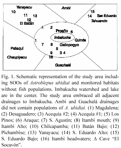
Study area. The study region (approximately 786 km2) is located in the south of the Province of Imbabura and a small portion of the north of the Province of Pichincha in the north of Ecuador, and encompasses must of the historic range of Astroblepus ubidiai (Barriga 1991). The core study area is the Imbakucha watershed (0º7 – 0º1542 N, 78º1032 – 78º1609 W), with a surface of 150.77 km2 and altitudes between 2661 m and 4400 m. Approximately 6% of the watershed area is occupied by Imbakucha Lake. The investigation included the study of adjacent drainages to Imbakucha: Tahuando, Ambi, Yanayacu, Chaupiyacu and Guachalá (Fig. 1). The borders of the study region match the species historic range and almost coincide with the area embraced by the lakes Yaguarcocha, Cuicocha, Mojanda and Imbakucha. All this portion of Imbabura is located above 2400 m altitude. The average annual temperature is 17ºC with a range of 15-30ºC (Ministerio de Relaciones Exteriores 1992, Kiersch and Muhleck 1997), and 15-20oC from November to June (Gunkel 1998, 2003, Kiersch et al. 2004).
The region presents an average annual precipitation of 1020.6 mm (Centro de Estudios Pluriculturales et al. 1999). The dry season runs from June to mid September, and the rainy season encompasses the last days of September to May, with strong rains during March, April and May.
Habitat inventory. Fieldwork involved the search for fish at all 30 sites where preñadilla were said to occur (12 within Imbakucha watershed and 18 in adjacent drainages) based on information gathered from interviews in communities within the region, and 22 sites based on the characteristics of habitat in the refuges. Habitat variables were assessed in sites of occurrence of the species and in a sample of 15 aquatic habitats without preñadilla, randomly selected from 34 aquatic bodies including springs, creeks, underground water, and first, second and third order streams where sampling indicated no presence of the fish. Nine of the selected sites were located at Imbakucha watershed, and the rest in the adjacent basins.
Fish were caught with D-nets, minnow traps and bag seine. Bag seine was used only in streams wider than 1m. Fish were released after the evaluation of weight and total length. Sites of occurrence were censused five times at intervals of approximately three months, and sites without preñadilla were monitored every two months during a 17-month period from June 2000 to November 2001.
Habitat Suitability Index HSI. The variables included in the HSI model are adapted from those used in the model developed for the white sucker, Catostomus commersoni, in the U.S.A. (Twomey et al. 1984). This model was chosen as a starting point because white sucker and preñadilla are both Siluriforms and present benthic behavior. The variables assayed to develop the model were current velocity, flow, depth, width, cover, invertebrate composition, vegetation type, terrestrial vegetation, land use, substrate, temperature, pH, total dissolved solids (TDS), oxygen, altitude, and slope were included in the analysis. Preñadillas HSI is also unique in part because it includes anthropogenic perturbations and the Fragment Isolation Index (FII) as habitat inventory variables.
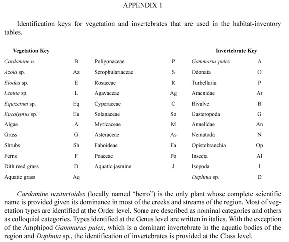
Oxygen concentration (mg/l) and percent saturation were estimated with a dissolved oxygen meter OXI 330 WTW. Values from the meter were certified by oxygen chemical determinations with a HACH chemical kit. The measurement of pH was made with a pH meter PH 330/Set-1 WTW. Performance of the electronic meter was corroborated with a HACH pH tester. Conductivity was measured with a LF 315 WTW meter. Total dissolved solids (TDS) were estimated from conductivity using a factor of 0.67, determined by Padilla (2000) for this region. The substrate classification utilized here is a mix of Cummings classification (Orth 1983), and Vadas and Orth (2001) average substratum size: mud, silt, sand, gravel, pebble, cobble, boulder, and bedrock. Current velocity was estimated with a Global Water flow probe FP 101 and corroborated with a floater. The flow or discharge (Q) was estimated by multiplying the average velocity v per the sum of the area cross sections (qi = depth * segment length): Q = v Σ qi. Percent of cover of aquatic vegetation was visually estimated from 15 x 60 cm quadrats (7 random throws per monitoring). The terrestrial vegetation variable refers to the vegetation located within 10 meters of the shoreline. Terrestrial vegetation is expected to be important to aquatic habitat as shading and a source of organic matter. Its composition was visually evaluated. Invertebrate taxon (Class or lower if possible) combined composition from the water column and substrate was evaluated utilizing D-nets. The sampling was undertaken upstream in the middle segment of the refuge for a 25 m distance. Nets were emptied every 5 m and organisms washed out in a 20 l bucket. Invertebrate taxa were classified as dominant (more than 50% frequency of occurrence in the overall sampling), sub-dominant (less than 50% of frequency of occurrence), and sporadic (less than 10% of frequency of occurrence) from visual inspection.
Anthropogenic perturbation index. Another variable considered as part of the habitat inventory was the human perturbation index (H), which is defined as the number of human perturbation types (identified in the reconnaissance study of February 2000) present in each site of occurrence or habitat divided by the total number of perturbation types (6), defined as following: (1) manipulation of the water flow, (2) point and non-point sources of organic water pollution, (3) clearing of aquatic vegetation at streams and creeks by communities, (4) fishing, (5) cattle perturbation, (6) introduction of exotics. These six kinds of anthropogenic perturbation have inexorable and continuous effects over fish populations, which do not show possibilities of escape as a consequence of habitat isolation. The timing and frequency of perturbation occurrence make them important and relatively constant environmental variables. These human perturbations affect habitat quality independently and interactively.
The Fragment Isolation Index (FII). Degree of habitat fragmentation is an important biogeographical variable that affects extinction process and trophic interactions. Loss and fragmentation of habitat result in reduced population size which increases the probability of extinction by demographic and/or environmental stochasticity (Fahrig 1997). The fragmentation of the habitat diminishes the resilience of fish. Some biogeographical variables related to habitat fragmentation and used in the conservation biology literature are the "total area of each fragment", and the "fragment isolation" measured as the distance to the closest fragment of equal or larger size (Crooks and Soulé 1999). The ratio between extent of occurrence and area of occupancy (terms proposed by the IUCN 2001) could eventually provide a measure of fragmentation. One of the new paradigms of conservation biology, the area-and-isolation paradigm has been validated by several taxa (Hanski 1998). Empirical data suggest that the probability of local extinction decreases as patch size increases, and that the probability of colonization increases as patch connectivity increases (Fleishman et al. 2002). The Fragment Isolation Index (FII) proposed here is a descriptor of a habitat fragments degree of isolation, and the radial distance to the closest patch represents the relative degree of connectivity. The FII is represented by the ratio between the area of the circle (A) in which the distance to the closest refuge (dcr) is the radius and the refuge area (A r). FII = ln (A / A r) = ln ( r2 / A r) = ln [(dcr)2 / Ar ].
FII will increase when dcr increases and/or when A r decreases. If the effect of patchiness is theoretically isolated, an inverse relationship is expected between FII and indicators of population performance such as density, biomass or Population Well-being Index PI (described later). The natural logarithm function in the FII formula smoothes scale effects. FII is used as a habitat inventory variable because the degree of fragmentation has been found to affect abundance and distribution (Fahrig 1997, Crooks and Soulé 1999). The FII can be applied to different species, and the significance of its value will be in relation to the life history and dispersal capacity of the species and the gene flow strategy used by the organisms.
Home range depends on the size and mobility of the fish, and population area depends on population size and lifestyle (Minns 1995). In some situations, the pattern of gene flow among colonies or patches is independent of relative geographical proximity (Lande and Barrowclough 1987). The dispersal of freshwater fishes is dependent on direct connections between drainage basins. These connections may include groundwater and temporal drainages. The FII corresponds more to an island biogeography model of population structure. If the average dispersal distance for the species is low relative to average distance between patches (or refuges), the spatial habitat structure can have an important limiting impact on local population size (Fahrig and Paloheimo 1988).
Biomass density and Population Wellbeing Index. Abundance was estimated using the Weighted Mean variant of the Petersen capture recapture method (Begon 1979) during three consecutive days. Fish were marked with a small clip in the caudal fin. Information on the size structure of biomass was estimated in every census for every site of occurrence as: B = Σ( Di x Wi ), where Di is the density of the size classes i and Wi is the average weight of the size class i. Within the context of the use of biomass density as a habitat quality indicator, and the production of healthy fishes as a reflection of productive capacity, Population Well-being Index (PI) was defined as a function of biomass density and health condition of the population in each refuge, as follows: PI = B(1- SF), where B= (refuge biomass density / maximum census biomass density) and SF = (fraction of sick fish in the population/ 2). B is biomass density scaled to values from 0 to 1. The division by 2 in SF calculation is due to the need to distribute the numeric weight between the two factors of PI equation (biomass and health condition). Fish health was evaluated by external observation of cysts, parasites, fungi, or deformities.
HSI calculation. Habitat inventory variables were measured not only for sites of occurrence (SOOs), but also for habitats where preñadilla was not present. This was done to detect critical values of variables. These are defined as the values, compositions or categories that limit the distribution (through negative effects) of the species. Critical values are detected empirically from habitats without the species and are recognized because their annual average or modes are found out of the variable range or categories obtained from SOOs.
The methodology to calculate the HIS includes eight steps: (1) Estimate PI for each refuge; (2) Obtain ranges and averages for each variable within each SOO; (3) Detect variables critical values from the habitats without preñadilla; (4) Perform correlation analysis on PI from every SOO and their single variable values, including the critical variable values from habitats without preñadilla present. If there is more than one critical value for a single variable the more extreme is included in the model. It is considered that PI = 0 for every critical value. Critical values may be normally distributed. For instance, low and high pH and temperature values can have a negative effect in fish. In such cases, only one of the sets of extreme values (the most distant from the mean) was included in the correlation. In one-tail negative effect cases, such as TDS, depth, or oxygen, only the extreme critical values with negative effects were included in the correlation; (5) Determine the Suitability Index (SI) for each variable: SI vn = PI (¦r¦vn = 0.6; p<0.1) where r vn is the Spearman rank correlation coefficient for variable n. Variables with ¦r¦< 0.6 were not included in the model. High r (~1) between independent variables represents a case of multicollinearity. In such cases only one variable was included in the calculation of the HSI; (6) SI for categorical variables such as type of substratum, type of vegetation and invertebrates composition was evaluated as following: SI vn = PI. In the cases when two different SOOs have the same type or composition, the mean of the PI was used to represent that type or composition. When the lack of correspondence between PI and independent categorical variable was obvious, that categorical variable was not included in the calculation of the HSI; (7) Perform linear regression after SI-arcsine transformation in order to develop SI equations for each variable (SI-transformed values – dependent variable; variable values – independent variable); (8) Calculation of the HSI for each site: HSI = (SIv1 x SIv2 x x SIvn )1/ n or HSI = (SIv1 + SIv2 + + SIvn ) / n in the cases when one or more SI values are "0".
Results
Population Well-being Index. The fish survey detected the presence of six preñadilla SOOs distributed in 4 different watersheds: three at Imbakucha (Proaño, Quinde and Gallopogyo), one at Tahuando (San Eduardo), one at Chaupiyacu (Pataquí), and one at Yanayacu (El Batán) (Fig. 1). The sites of occurrence of the target species within the Imbakucha watershed were located in an ecosystem influenced by the presence of the lake. The populations located in the adjacent drainages do not have the immediate connection with any kind of lentic system. Table 1 shows the final PI values for every refuge. El Batán was the refuge with the highest PI value (0.7968). It is interesting that the three lowest PI values correspond with the refuges within Imbakucha watershed (Proaño, Gallopogyo and Quinde). In this watershed all six anthropogenic perturbations occur in the refuges. Approximately 30 000 inhabitants distributed in 38 communities within an area of 150 km2, have doubtless impacted on preñadilla habitat, and it partly explains the poor Population Wellbeing Index values.
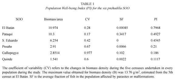
The population with the biggest SF value was Pataquí (0.3417) affected with an endoparasite (trematode) similar to the black spot present in North American fish. Other affections observed in preñadilla in other refuges were exoparasites (arthropoda) and some deformities of the vertebral column.
Habitat variables. Habitat was measured at six preñadilla refuges and 15 aquatic habitats without preñadilla populations (Fig. 1). The annual mean values of the habitat variables and their critical values detected from the sample of sites without the fish are shown in Table 2. The dominant compositions of categorical variables in the refuges and their critical compositions from selected habitats are presented in Table 3.
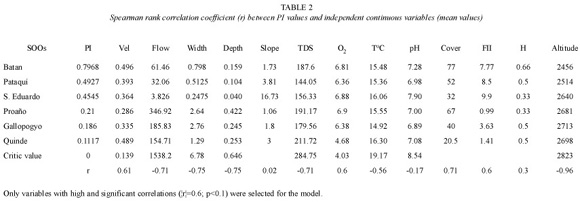
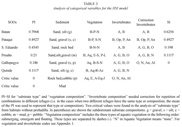
Table 2 also shows the values of r before eliminating the variables with values of |r|<0.6. A marginal significance is used in the statistical filter given the small size sample (6 variable values from SOOs plus critical value), which makes a high significance very restrictive, independently of the intensity of the association between the two variables indicated by r. A very high correlation (r=0.99; p<0.05) between the variables flow and depth (both with r >0.6 in relation to PI) supported the elimination of the variable flow from the model given that flow is the result of velocity and geometry in the system, and the outcome of correlation analysis selected velocity, width, and depth as determinant habitat variables.
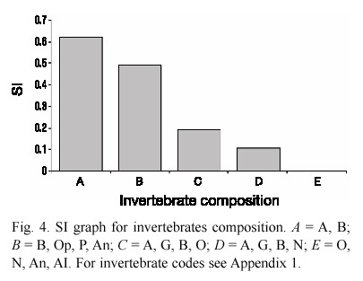
Not all variables in Table 3 data series have critical values. According to the methodology, PI=0 corresponded with every critical value. Categorical variables followed a different analysis (step 6). The variables "land use" and "terrestrial vegetation" were eliminated for lack of correspondence with the changes in PI: pasture ground is a constant in all the refuges, and the combination G, Sh is the kind of terrestrial vegetation present in all the refuges (see vegetation and invertebrate codes in Appendix 1). Substrate type and vegetation did not repeat between refuges, and did not need correction for repetition. However, correction was needed for "invertebrate composition" (step 6) where the combinations A, B and A, G, B, O were repeated. For that reason only five invertebrate compositions remained. Table 3 displays these categorical variables and the correction performed.
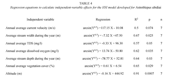
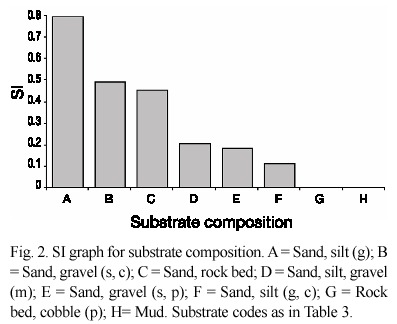
From the eighteen variables assayed during the study only 10 prevailed to be included in the final step of the HSI model. These variables were: velocity, depth, width, TDS, oxygen, altitude, percentage of aquatic vegetation, aquatic vegetation composition, substrate, and invertebrates composition. The correlation with FII (r=0.6) was not considered as affecting habitat suitability because according to the definition it was expected an inverse relationship between PI and FII. Unfortunately, the correlation is positive and lacks ecological significance. The highest PI correlation with continuous variables was that with altitude (r = -0.96; p=0.0004). The regressions and SI graphs exhibited in Table 4 and figures 2, 3 and 4 respectively are the very last product of the HSI model developed for A. ubidiai. Now these graphs and regressions become the main tool to estimate the suitability of aquatic lotic habitats for the target species. The final HSI values for the refuges were 0.78, 0.49, 0.47, 0.21, 0.19, and 0.11 for El Batán, Pataquí, San Eduardo, Proaño, Gallopogyo, and Quinde respectively. The similarity between the HSIs and the PI values estimated for refuges is because SIs values are PI-based, meaning they depend on the biomass density and health found in every population. However, HSI values for the refuges are not the important output of the model but the possibility of measuring the habitat suitability from other habitats.

Estimation of HSI from diverse habitats. HSI values range from 0 to 1. In this study, habitat is rated arbitrarily in terms of quality as follows: low quality (HSI ≤ 0.2), medium quality (0.2 < HSI = 0.5), good quality (0.5 < HSI = 0.8), and high quality (HIS > 0.8). In Table 5 are displayed the HSIs for the habitats without fish populations surveyed during this investigation. None of these habitats contained preñadilla but were studied for the detection of critical values of variables, to assess a representative sample of the aquatic habitats within the study area, and to have and idea of the availability of good quality habitat for potential introductions.
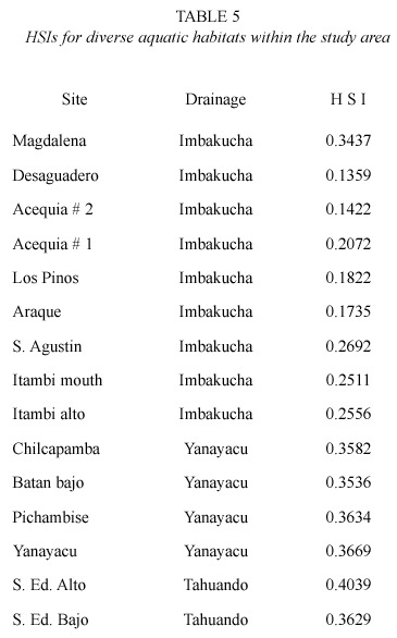
The survey revealed that 26.6% of the unoccupied habitats were of low quality, and the rest (73.4%) were of medium quality. These 15 surveyed habitats are a representative sample of the actual available habitat in the study area because they were randomly selected from 34 aquatic bodies in the study region. Although the search for preñadilla at the beginning of the study included the main lakes of the study region (Imbakucha, Yaguarkucha, Cuicocha, and Mojanda), they were not considered as potentially suitable habitats given the lack of evidences indicating the presence of A. ubidiai in lentic habitats (Vélez-Espino 2003a).
Discussion
The present HSI model can be defined as an interactive assessment (Vadas and Orth 2001) model because it is incorporating biotic as well as physical habitat variables. The regression equations of the selected continuous variables had good statistical significance, with the exception of average current velocity, which produced a marginally significant regression. These results support the use of arcsine-transformed data for y values ranging from 0 to 1 as is the case of the SI scale used in this model. Another factor that influenced the good performance of regressions was the previous filter through correlation analysis. This step allowed the selection of the principal environmental components influencing population performance in terms of biomass density and health.
The non-significant observed relationship between the fragment isolation index (FII) and the population well-being index (PI) is explained in terms of the high degree of isolation represented by the studied populations. The hypothesis of a positive relationship between FII and PI is based in the assumption that distance and refuge size are affecting the migration rates. But when the lack of connectivity among refuges is independent of these factors, the effect of FII on abundance or biomass density is not detectable.
The six study populations are distributed in four different drainages (Fig. 1), and their probabilities to escape to other refuges when the environment deteriorates seems very limited due to natural barriers between drainages. Pasture grounds, fields, human settlements, and the presence of the piscivorous largemouth bass Micropterus salmoides in Imbakucha Lake (Vélez- Espino 2003a) separate the populations within the watershed. In other words, each population seems to be demographically independent. The effect of human perturbations as a habitat variable could be better interpreted if it is included in the anthropogenic perturbation index H a measure of the frequency and intensity of perturbations. The lack of these elements in the definition of H may be one of the reasons why there was not a significant correlation with PI.
The high intensity of the association between altitude and SI, determined by a very high and significant correlation, was very surprising. In fact, the regression analysis exhibited a strong linearity, and similar HSI values are obtained with estimates of altitude alone. Definitely altitude is a very important habitat variable but it is not sufficient to evaluate habitat suitability. The negative correlation between altitude and SI allow the conclusion that unfortunately for the species, the weakness of the anthropogenic forces in uninhabited places in high elevations may not benefit A. ubidiai.
The understanding of habitat quality and its implications for metapopulation dynamics may clarify the importance of habitat protection or restoration as effective management strategies (Fleishman et al. 2002). The probability of metapopulation extinction depends on the number, size, quality and connectivity of habitat fragments in the system (Drechsler and Wissel 1998). Deterioration of habitat quality and quantity can affect population size, distribution, and response to a perturbation. Habitat quality interacts with the population phenotype to establish the population density or carrying capacity.
As are many of the species that are subject to population viability analysis, Astroblepus ubidiai is restricted to island-like habitats. The measurement of habitat quality in current refuges allowed the verification whether or not remnant populations are occupying the habitat most favorable or the habitat least favorable to the agent of decline. Caughley (1994) suggested the latter assumption as a safer preliminary hypothesis compared with assuming that the remnants of the species are in the most favorable habitat. The fact that the habitats of all populations are either springs or headwaters is probably not because those are the keystone habitats, but because those are the habitats least favorable to the agent(s) of decline (which can be all the listed anthropogenic perturbations). The low HSIs within Imbakucha, which are linked to the high level of anthropogenic perturbations in the watershed, support this assumption. None of the nine surveyed sites within the Imbakucha watershed, which could serve as refuges during perturbations or could be used as rescue spots for translocations, offers good quality. All have HSIs below 0.4. Higher HSIs were estimated in the adjacent drainages to Imbakucha, but area of occupancy was still limited to the springs and headwaters surrounding area. These results suggest that remnant populations are located in refuges that provide certain resilience to habitat destruction and deterioration. The same stability is provided to fish populations by desert springs, which usually present constant discharge rate, water level, temperature, TDS, and oxygen during long periods (Naiman 1981).
It is important to mention that preñadillas use of underground refuges was mentioned by Humboldt and Bonpland (1805). I observed the faculty of preñadilla of going into interstitial spaces and disappear through the mouth of springs. The importance of underground water in the life cycle of the species is unknown, but the genus Astroblepus is known to have troglobitic (exclusively subterranean) and troglophilic (facultative subterranean) species. Astroblepus riberae (Cardona and Guerao 1994) collected in Ninabamba caves, Cajamarca, Peru, and Astroblepus pholeter (Collette 1962) collected in the Jumandi Cave, Napo province, Ecuador, have been formally described as hypogean fishes (Romero and Paulson 2001). More research is needed to understand the importance of subterranean water in the life cycle and resilience of Astroblepus ubidiai to habitat perturbations. The role of underground water as shelter under adverse environmental conditions would partially explain the large biomassdensity coefficients of variation (Table 1) in refuges, especially in those within Imbakucha watershed. The possibility of migration as an explanation for population size fluctuations between censuses is low for four reasons: (1) the degree of fragmentation of the habitat; (2) high recapture rates during the study; (3) documented sedentary behavior and site fidelity in troglobitic and troglophile species (Trajano 2001); and (4) the few organisms sampled out of refuges.
Extinction factors may have synergistic effects (Mace and Lande 1991). For example, overfishing may not have been a problem before the population was fragmented by habitat loss. Now the concentration of fish in a few small localities increases the vulnerability of preñadilla and jeopardizes the population. The current fragmentation between populations within the Imbakucha watershed has been enhanced by the introduction of exotics. Standard anthropogenic perturbations are the deviation of water currents towards pasture grounds, the periodic vegetation clearing from creeks by communities in order to improve the water supply, the use of preñadilla as bait for largemouth fishing, the old custom of cloth washing in the water in springs, creeks and streams, and the old custom also of using aquatic bodies as corridors to walk the cattle within the watershed.
Fish passage is another limiting factor in the study region. All populations are isolated geographically, by human settlements and due to arbitrary water use. The low probability that dispersers successfully reach other refuges hinders a positive effect of migration on the regional population size (Fahrig and Paloheimo 1988). During the recovery of the traditional ecological knowledge it was surprising that five of former preñadilla habitats were converted in reservoirs for human supply and floriculture, four were transformed to community-washing places, two were dried as a consequence of inappropriate agricultural activities, and one was converted in religious sanctuary as it is the case of the cave called "El Socavón" (Fig. 1), which traditional knowledge recognized as a former source of preñadilla. The use of the local agave called "cabuya" (Cactaceae) in the washing of clothes in the creeks and streams is known to have active chemical substances that kill aquatic fauna, including fish (L.A. Vélez, personal observation).
The availability of the HSI model for Astroblepus ubidiai has important implications for the conservation of the species. It will allow measuring the degree of deterioration or amelioration (if conservation actions are effectively implemented) in current refuges by undertaking periodic estimations of HSI. For instance, habitat rehabilitation actions are being implemented in a former preñadilla refuge, Araque springs, (Fig. 1) within the Imbakucha watershed by local researchers involved in the present investigation. A. ubidiai was recently extirpated from this site and the effect of habitat restoration will be monitored with the HSI developed here in order to evaluate the suitability of the habitat as a spot for potential translocations.
Other application of the HSI developed for A. ubidiai is its usefulness for the evaluation of habitat quality as a criterion for the categorization of extinction threats. The IUCN recognizes that taxa that are poorly known can be assigned a threat category on the basis of habitat deterioration (IUCN 2001). Using the present model it was established that, with the exception of El Batán, the rest of preñadilla populations meet the criterion for vulnerable or endangered (Vélez-Espino 2003b).
The persistence of this unique Andean fish depends strongly in our understanding of its essential habitat and the capacity to measure habitat-quality trends whether they are the result of management or the consequence of the environmental impact produced by human activities.
Acknowledgments
This work was supported by a doctorate award from "El Consejo Nacional de Ciencia y Tecnología" from Mexico (CONACYT), and by the CIDA-funded Tier 1project INSTRUCT. I am very grateful to T. Whillans for his helpful comments on an earlier version of this manuscript.
Resumen
Astroblepus ubidiai (Siluriformes), el único pez nativo de las alturas de Imbabura, en los Andes Ecuatorianos, era un recurso abundante en el pasado. Actualmente su distribución está limitada a unos cuantos refugios aislados. Se necesitan acciones de conservación para que esta especie perdure. Se desarrolló un modelo para estimar el índice de calidad de hábitat (ICH) que ayude en futuras decisiones de manejo. En este ICH la densidad de biomasa (B) fue seleccionada como un mejor indicador de calidad de hábitat, comparada con el uso común de abundancia o densidad incorporado en otros modelos. Se generó un índice de bienestar poblacional (IP) basado en B y en un indicador de salud poblacional (SP) derivado de la proporción de peces en la población con parásitos y malformaciones. Diecinueve variables físicas, biológicas y geográficas fueron evaluadas dentro del modelo, el cual fue aplicado a una muestra de 15 sitios sin poblaciones de A. ubidiai dentro del área de estudio. De esta muestra, 26.6% de los sitios presentó baja calidad de hábitat, y el restante 73.3% presentó calidad media de acuerdo a la evaluación con el modelo. En la región hay escasos hábitats de buena calidad para dispersión, escape y reubicación de este pez.
Palabras clave: Astroblepus ubidiai, preñadilla, calidad del hábitat, inventario del habitat, fragmentación.
References
Anderson, P.G. 1993. Adaptation of a habitat suitability model for prioritizing habitat rehabilitation needs for northern pike (Essox lucius). M. SC. Thesis. Trent University, Peterborough, Ontario, Canada. 147 p. [ Links ]
Barriga, R. 1991. Peces de agua dulce del Ecuador. Revista de información técnico científica (politécnica), 3: 51- 71. Escuela Politécnica del Ecuador, Quito, Ecuador. [ Links ]
Begon, M. 1979. Investigating animal abundance: capturerecapture for biologists. University Park, Baltimore, Ohio, USA. 97 p. [ Links ]
Boudreau, P.R. & L.M. Dickie. 1989. A biological model of fisheries production based on physiological and ecological scalings of body size. Can. J. Fish. Aquat. Sci. 46: 614-623. [ Links ]
Boudreau, P.R., & L.M. Dickie. 1992. Biomass spectra of aquatic ecosystems in relation to fisheries yield. Can. J. Fish. Aquat. Sci. 49: 1528-1538. [ Links ]
Bovee, K.D. 1986. Development and evaluation of habitat suitability criteria for use in the instream inflow incremental methodology. Instream Flow Information Paper 21. U.S. Fish and Wildlife Service Biol. Rep. 86(7): 1-235. [ Links ]
Cardona, L. & G. Guerao. 1994. Astroblepus riberae, una nueva especie de siluriforme cavernícola del Perú (Osteichthyes, Astroblepidae). Mem. Biospeleol. 12: 21-24. [ Links ]
Caughley, G. 1994. Directions in conservation biology. J. Animal Ecol. 63: 215-244. [ Links ]
Centro de Estudios Pluriculturales CEPCU, Programa de las Naciones Unidas para el Desarrollo PNUD, Voluntarios de las Naciones Unidas VNU, Inter- American Network for Studies and Training in (Natural) Resource Usage for Community Transformation INSTRUCT, Consejo de Desarrollo de las Nacionalidades de los Pueblos del Ecuador CODENPE. 1999. Plan de Manejo Integrado de la Cuenca del Imbakucha. Otavalo, Ecuador. 87 p. [ Links ]
Collette, B.B. 1962. Astroblepus pholeter, a new species of cave dwelling catfish from Eastern Ecuador. Proc. Biol. Soc. Washington. 75: 311-314. [ Links ]
Crooks, K.R. & M.E. Soulé. 1999. Mesopredator release and avifaunal extinctions in a fragmented system. Nature 400: 563-566. [ Links ]
Dodson, J.J., R.J. Gibson, R.A. Cunjak, K.D. Friedland, C. García de Leaniz, M.R. Gross, R. Newbury. J.L. Nielsen, M.E. Power & S. Roy. 1998. Elements in the development of conservation plans for Atlantic salmon (Salmo salar). Can. J. Aquat. Sci. 55 (Suppl. 1): 312-323. [ Links ]
Drechsler, M. & C. Wissel. 1998. Trade-offs between local and regional scale management of metapopulations. Biol. Conserv. 83: 31-41. [ Links ]
Fahrig, L. & J. Paloheimo. 1988. Determinants of local population size in patchy habitats. Theor. Pop. Biol. 34: 194-213. [ Links ]
Fahrig, L. 1997. Relative effects of habitat loss and fragmentation on population extinction. J. Wildl. Manage. 61(3): 603-610. [ Links ]
Fleishman, E., C. Ray, P. Sjogren-Gulve, C.L. Boggs, & D. Murphy. 2002. Assessing the roles of patch quality, area, and isolation in predicting metapopulation dynamics. Conserv. Biol. 16: 706-716. [ Links ]
Gilpin, M.E. & M.E. Soulé. 1986. Minimum viable populations: processes of species Extinction, p. 19-34. In M.E. Soulé (ed.). Conservation Biology: The science of scarcity and diversity. Sinauer Associates, Sunderland, Massachussetts, USA. [ Links ]
Gore, J.A. 1989. Models for predicting benthic macroinvertebrate habitat suitability under regulated flows, p. 253-265. In J.A. Gore & G.E. Petts (eds.). Alternatives in regulated river management. CRC, Boca Raton, Florida, USA. [ Links ]
Gunkel, G. 1998. Eutroficación del Lago San Pablo. Limnología y protección de ecosistemas acuáticos. Centro de Educación Contínua del Instituto de Postgrado. Escuela Politécnica Nacional, y Technical University of Berlin. Quito. 13 p. [ Links ]
Gunkel, G. 2003. Limnología de un lago tropical de alta montaña, en Ecuador: Características de los sedimentos y tasa de sedimentación. Rev. Biol. Trop. 51: 381-390. [ Links ]
Hanski, I. 1998. Metapopulation dynamics. Nature 396: 41-49. [ Links ]
Harris, A.G., S.C. McMurray, P.W.C. Uhlig, J.K. Jeglum, R.F. Foster & G.D. Racey. 1996. Field guide to the wetland ecosystem classification for Northwestern Ontario. Ministry of Natural Resources, Ontario. Canada. 22 p. [ Links ]
Humboldt, A. & A. Bonpland. 1805. Recueil dobservations de zoologie et danatomie comparée. Paris. p. 39-46. [ Links ]
IUCN. 2001. IUCN Red List Categories and Criteria: Version 3.1.IUCN Species Survival Commission. IUCN, Gland, Switzerland. 30 p. [ Links ]
Jones, M.L., R.G. Randall, D. Hayes, W. Dunlop, J. Imhof, G. Lacroix & N.J.R. Ward. 1996. Assessing the ecological effects of habitat change: moving beyond productive capacity. Can. J. Fish. Aquat. Sci. 53 (Suppl. 1): 446-457. [ Links ]
Kiersch, B. & R. Muhleck. 1997. Caracterización de la vegetación de macrofitas en los lagos de San Pablo, Cuicocha y La Mica (Sierra Andina Ecuatoriana). Technical University of Berlin. Department of water control. Berlin. 25 p. [ Links ]
Kiersch, B. & R. Muhleck & G. Gunkel. 2004. Las macróficas de algunos lagos alto-andinos del Ecuador y su bajo potencial como bioindicadores de eutroficación. Rev. Biol. Trop. 52: 829-837. [ Links ]
Lande, R. & G.F. Barrowclough, 1987. Effective population size, genetic variation, and their use in population management, p. 86-123. In M.E. Soulé (ed.). Viable populations for conservation. Cambridge University, Cambridge, England [ Links ]
Leclerc, M., A. Boudreault, J.A. Bechara & G. Corba. 1995. Two-dimensional hydrodynamic modeling: a neglected tool in the instream flow incremental methodology. Trans. Am. Fish. Soc. 124: 645-662. [ Links ]
Li, H.W., C.B. Schreck & K.J. Rodnick. 1984. Assessment of habitat quality models for cutthroat trout and coho salmon for Oregons coastal streams, p. 57-111. In J.W Terrel (ed.). Proceedings of a workshop on fish habitat suitability index models. U.S. Department of the Interior, U.S. Fish and Wildlife Service. Washington D.C., Biological Report, 85(6). [ Links ]
Mace, G.M. & R. Lande. 1991. Assessing extinction threats: toward a reevaluation of IUCN threatened species categories. Conserv. Biol. 5: 148-157. [ Links ]
Ministerio de Relaciones Exteriores. 1992. Estudio para la recuperación y protección de la zona turística de los Lagos de la Provincia de Imbabura con fines de equilibrio ecológico y promoción turística. Informe General. Ecuador. 154 p. [ Links ]
Minns, C.K. 1995. Allometry of home range in lake and river fishes: body size and ecosystem type. Can. J. Fish. Aquat. Sci. 52: 1499-1508. [ Links ]
Minns, C.K., J.R.M. Kelso & R.G. Randall. 1996. Detecting the response of fish to habitat alterations in freshwater ecosystems. Can. J. Fish. Aquat. Sci. 53 (suppl.1): 403-414. [ Links ]
Minns, C.K., S.E. Doka, C.N. Bakelaar, P.C.E. Brunette & W.M. Schertzer. 1999. Identifying Habitats essential for pike Esox lucius L. in the Long Point region of Lake Erie: a suitable supply approach, p. 363- 382. In L.R. Benaka (ed.). Fish Habitat: Essential Fish Habitat and Rehabilitation. American Fisheries Society, Symposium 22. [ Links ]
Naiman, R.J. 1981. An ecosystem overview: Desert fishes and their habitats. p. 493-531. In R.J. Naiman & D.L. Soltz (eds.). Fishes of the North American Deserts. Wiley, New York, USA. [ Links ]
Orth, D.J. 1983. Aquatic habitat measurements, p. 61- 83. In L.A. Nielsen & D.L. Johnson (eds.). Fisheries techniques. American Fisheries Society. Bethesda, Maryland, USA [ Links ]
Padilla Villacís, A.C. 2000. Evaluación ambiental de la microcuenca del río Itambi. Tesis de Licenciatura en Ciencias Geográficas y Estudios Ambientales. PUCE. Quito. 130 p. [ Links ]
Randall, R.G., J.R.M. Kelso & C.K. Minns. 1995. Fish production in freshwaters: are rivers more productive than lakes? Can. J. Fish. Aquat. Sci. 52: 631-643. [ Links ]
Romero, A. & K.M. Paulson. 2001. Its a wonderful hypogean life: a guide to the troglomorphic fishes of the world. Env. Biol. Fish. 62: 13-41. [ Links ]
Rubec, P.J., J.C.W. Bexley, H. Norris, M.S. Coyne, M.E. Monaco, S.G. Smith & J.S. Ault. 1999. Suitability modeling to delineate habitat essential to sustainable fisheries, p. 108-133. In L.R. Benaka (ed.). Fish Habitat: Essential Fish Habitat and Rehabilitation. American Fisheries Society, Symposium 22. [ Links ]
Stephens, P.A. & W.J. Sutherland. 1999. Consequences of the Allee effect for behavior, ecology and conservation. Trends Ecol. Evol. 14: 401-410. [ Links ]
Stuber, R.J., G. Gebhart & O.E. Maughan. 1982. Habitat Suitability Index Models: largemouth bass. Fish and Wildlife Service. U.S. Department of the Interior. Washington, DC. 27 p. [ Links ]
Terrel, J.W. 1984. Proceedings of a workshop on fish habitat suitability index models. U.S. Fish and Wildlife Service Biol. Rep. 85(6): 1-393. [ Links ]
Trajano, E. 2001. Ecology of subterranean fishes: an overview. Env. Biol. Fish. 62: 133-160. [ Links ]
Twomey, K.A., P.C. Nelson & C. Armour. 1984. Habitat suitability index models and instream flow suitability curves: white sucker. Fish and Wildlife Service. U.S. Department of the Interior. Washington, DC. 56 p. [ Links ]
Vadas, R.L. & D.J. Orth. 2001. Formulation of Habitat Suitability Models for stream fish guilds: do the standard methods work? Trans. Am. Fish. Soc. 130: 217-235. [ Links ]
Vélez-Espino, L.A. 2003a. Ecology and conservation biology of the Andean catfish Astroblepus ubidiai in the highlands of Imbabura Province, Ecuador. Ph. D. Thesis. Trent University, Peterborough, Ontario, Canada. 325 p. [ Links ]
Vélez-Espino, L.A. 2003b. Taxonomic revision, ecology and endangerment categorization of the Andean catfish Astroblepus ubidai (Teleostei: Astroblepidae). Rev. Fish Biol. Fisheries: 13: 367-378. [ Links ]
Zar, J.H. 1999. Biostatistical analysis. Prentice Hall, New Jersey, USA. 663 p. [ Links ]

