


 English (pdf)
 Article in xml format
 Article references
 Send this article by e-mail
 Cited by SciELO
  Similars in
SciELO
Similars in
SciELO  uBio
uBio 
 Permalink
Introduction
Harmful proliferations of algae and cyanobacteria are globally recognized for their economic, health and environmental impacts; and the overall degradation of resource quality (Kudela et al., 2017). These are an increasing phenomenon, and their occurrence is consistently expanding into new areas (Cheung et al., 2013).
In the case of cyanobacterial blooms (CB), which could be associated with toxin release, their risk assessment continues to be a challenge. The World Health Organization establishes guideline levels for cyanobacteria based on cell concentrations (World Health Organization, 2003), which serve as a basis for cyanobacterial risk assessment. However, most countries lack specific regulations and pay attention when it is too late.
The relationship between CB and abiotic factors is well-documented since it has been the focal point for researchers over numerous years. Investigations have primarily concentrated on local abiotic factors such as temperature, light conditions, nutrient concentrations and their ratios, pH, and conductivity (O’Neil et al., 2012; Paerl & Otten, 2013; Paerl & Otten, 2016). However, the impact of these events on the rest of the phytoplankton community and biological parameters is much less understood, and little is known about possible early biological warnings. It has been previously postulated that the establishment of CB could be associated with other interactions within the community beyond nutrient competition (Kokociński et al., 2021) but this biological standpoint has been poorly explored until today.
Co-occurrence and/or correlation abundance networks emerge as intriguing tools to comprehend species interactions (D’Amen et al., 2018). These networks could unveil interaction patterns and novel insights into potential connections among various species (Berry & Widder, 2014). In general, they are employed to explore how microbial interactions respond to environmental disturbances and are widely used in microbiome research (Lu et al., 2022) but have been little used in phytoplanktonic communities. Lozano (2022) has explored the possibility of using correlation abundance networks as an early tool for assessing the impact of herbicidal in freshwater ecosystems with promising results. Biological interactions could be manifested in the structure of co-occurrence networks (Rüger et al., 2021) and, in the case of correlation of abundance networks, positive correlation could be associated with taxa acting similarly, cooperation, facilitation, mutualism, and symbiosis, while negative correlations could be associated to competition and/or taxa presenting opposing behaviors (Lozano, 2022). Although such networks must reflect these biological interactions, further research is needed to verify this correspondence, since correlations can show artifacts (Feng et al., 2019; Lozano, 2022). Nevertheless, considering both abiotic and biotic interactions is fundamental to a better comprehension of CB and both need to be assessed.
To test the possibility of using the correlation of abundance networks as an early alert tool for CB, we analyzed 4 levels of CB in a tropical reservoir in Argentina.
Materials and methods
Study area: El Limón (22°6’12.29’’ S & 63°44’21.34’’ W) reservoir is in the Northern province of Salta, Argentina. It covers approximately 100 ha with a capacity of 1.7 Hm3, and an average depth of 4 m. The climate in the area is distinctly tropical with high temperatures during the dry season and an annual average rainfall exceeding 970 mm (Arias & Bianchi, 1996). The average altitude of the region stands at 550 m.a.s.l. in an area referred to as the “piedmont” or “transitional jungle”.
Sampling: Between June 2018 and January 2020, a total of 22 samples (in 1 l bottles) were collected monthly in the El Limón reservoir at the Secchi depth. Additionally, some bimonthly samplings were conducted during the warmer months, as they are associated with periods of bloom development. The sampling site remained constant at the only access point to the Reservoir, situated approximately 15 m from the shoreline (Fig. 1).
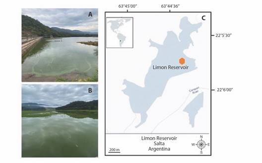
Fig. 1 El Limón Reservoir and pictures of the study area. A. and B. Photographs of the El Limón Reservoir. C. Study area map, the orange dot in the reservoir marks the sampling site.
Taxonomic phytoplankton counting: For phytoplankton analysis, qualitative samples were collected below the surface using a 30 µm mesh net, that was dragged horizontally, and fixed with 4% formaldehyde. Formaldehyde-fixed samples were used solely for support purposes in taxonomic identification. Quantitative analysis was carried out using samples taken at the depth of a Secchi disk, fixed in acidified Lugol’s solution, and stored at 4 °C until analysis. After 24 h of sedimentation, counts were performed using combined chambers on an inverted Zeiss L microscope, following the method by Utermöhl (1958). Each sample was counted to obtain less than a 20% error for the most frequent species (Venrick, 1978). The results were expressed in cells/ml. The number of cells per filament was determined by dividing the total filament length by the mean cell length (N= 20). Organisms without cellular content were excluded from the count. Species were identified by capturing images using an Axio Cam1Cc3 digital camera and utilizing specialized references such as Komárek and Anagnostidis (1999), Komárek and Anagnostidis (2005), Komárek (2014), Komárková-Legnerová (1969), Krammer and Lange-Bertalot (1986), among others.
In this study, a CB was considered when the abundance of at least one species of cyanobacteria exceeded 5 000 cells/ml. Based on total cyanobacterial abundances, each sample was classified into different categories or levels. Four levels were pre-established based on total abundances (cells/ml): Level 1 (10 000-30 000); Level 2 (30 000-50 000); Level 3 (50 000-100 000); and Level 4 (> 100 000).
Physical and Chemical Variables: In all collections, a thermal profile of the reservoir was conducted. In-situ measurements were taken for temperature (°C), electrical conductivity (µs/cm), pH, and dissolved oxygen (D.O.) (mg/l) using an Orion multiparameter sensor. Additionally, turbidity was measured using a HACH turbidimeter (NTU), and transparency was assessed with a Secchi disk. Samples for physical and chemical analyses were collected using a Van Dorn sampler at the depth of 1- Secchi disk and refrigerated until analysis. Total and suspended solids (mg/l), true color, nitrates, nitrites, and ammonium (mg N/l), soluble reactive phosphorus (mg PRS/l), chemical oxygen demand (mg O2 /l), alkalinity (mg CaCO3/l), and hardness (mg CaCO3/l) were determined in the laboratory following standardized APHA techniques (APHA, 2005). Chlorophyll a concentration was measured using the modified Scor-Unesco technique (Cabrera-Silva, 1984). The trophic state of the reservoir was assessed using the Carlson Trophic State Index (TSI) based on chlorophyll a (Carlson, 1977).
Statistical Analysis: Using specific phytoplanktonic abundances by level, Spearman correlation coefficients were calculated using InfoStat v.2008 (Di Rienzo et al., 2010) and correlation of abundances networks were constructed using Cytoscape v.3.7.1. (Shannon et al., 2003), considering only significant correlation coefficients (P ≤ 0.01). The physical and chemical variables were compared between levels using the Kruskal-Wallis non-parametric test because variables did not meet the normality and/or homogeneity requirements.
Results
Based on the proposed classification of levels, the 22 samplings were divided as follows: 4 categorized in level 1; 8 in level 2; 5 in level 3; and 5 in level 4. Water temperature was statistically different among the 4 levels (H = 9.22, P = 0.0263). A trend of increasing temperatures during the CB classified in the higher levels was observed. Samplings classified in level 1 exhibited the lowest average air temperature (19.4 ± 6.01 °C), while those in level 4 recorded the highest average temperature in samplings (26.6 ± 2.84 °C). A similar pattern was observed in the water temperature of the reservoir, with means of 20.18 °C (± 4.95), 24.3 °C (± 2.84), 24.92 °C (± 6.69), and 31.98 °C (± 4.15) in levels 1, 2, 3, and 4, respectively.
Besides water temperature, the only water chemistry parameter significantly different between the levels was alkalinity (H = 8.84, P = 0.0314). Other parameters remained relatively stable throughout the analyzed period (Table 1).
Table 1 Average and standard deviations of physical and chemical variables for each level.
| Variable | Level 1 | Level 2 | Level 3 | Level 4 | Statistical differences |
| pH | 7.53 ± 0.64 | 7.18 ± 0.41 | 7.45 ± 0.44 | 7.29 ± 0.72 | (H = 1.63, P = 0.652) |
| E.C. (µS/cm) | 610.4 ± 32.7 | 547.6 ± 122.8 | 457.4 ± 168.4 | 600.9 ± 62.1 | (H = 3.23, P = 0.356) |
| Turbidity (NTU) | 3.14 ± 1.67 | 7.26 ± 6.87 | 3.88 ± 2.13 | 4 ± 1.78 | (H = 4.51, P = 0.211) |
| Alkalinity (mg CaCO3/l) | 132.3 ± 92.4 | 86.7 ± 14.4 | 153.7 ± 68.7 | 205.1 ± 27.1 | (H = 8.84, P = 0.031) |
| Hardness (mg CaCO3/l) | 217.9 ± 50.2 | 434.0 ± 549.4 | 275.2 ± 114.1 | 164.6 ± 51.4 | (H = 6.01, P = 0.111) |
| N/P | 17.6 ± 6.6 | 24.0 ± 30.3 | 16.42 ± 4.0 | 9.7 ± 7.4 | (H = 2.92, P = 0.404) |
| D.O. (mg O2/l) | 9.35 ± 1.40 | 8.77 ± 2.39 | 8.98 ± 1.52 | 8.04 ± 1.82 | (H = 1.10, P = 0.777) |
| T (°C) | 20.1 ± 4.9 | 24. ± 2.84 | 24.92±6.69 | 31.98 ± 4.15 | (H = 9.22, P = 0.026) |
The Carlson trophic index was calculated for all samplings based on chlorophyll a. The overall state of the reservoir was found to be mesotrophic, with only 3 eutrophic samplings corresponding to samplings in levels 1 and 2 in the wet season when the water level was 0.5 m superior to the average (4 m). Regarding phytoplanktonic species richness over the entire considered period, 162 species were identified. The most important group was the Chlorophyceae with 65 spp., followed by Cyanobacteria with 51 spp. Additionally, 22 species of Bacillariophyceae, 11 of Euglenophyceae, 5 of Cryptophyceae, and 3 of Dinophyceae were identified.
Species richness was 66 spp. in level 1, 83 spp. in level 2, 56 spp. in level 3, and 42 spp. in level 4. The highest richness of cyanobacteria was observed in level 2 (41 spp.), followed by level 1 (33 spp.), despite their lower abundances compared to levels 3 and 4. Dominant cyanobacteria species in each level were Aphanocapsa elachista in level 1 and Raphidiopsis mediterranea in levels 2, 3, and 4. The Venn diagram in Fig. 2 illustrates the species that overlap between different levels and those exclusive to each one. 27 species were found at all levels. Specifically, level 1 documented 9 exclusive species, while 11, 3 and 1 were exclusive to levels 2, 3 and 4 respectively.
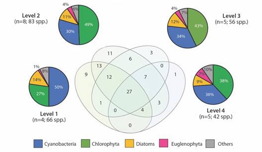
Fig. 2 Phytoplanktonic richness in the different levels. Venn diagram shows the species shared between levels. Pie charts show the species classification in broad taxonomic groups.
Total phytoplankton abundances showed statistically significant differences (H = 19.1, P = 0.0003). A sustained increase in total phytoplankton abundance was observed at higher levels. In this regard, the phytoplankton abundance in level 4 was 1 117 % higher than the average total abundance recorded in level 1, corresponding level 4 to the most intense blooms. Cyanobacterial mean abundances values were: 18 693 (± 5 787 cells/ml), 38 188 (± 6 968 cells/ml), 62 924 (± 15 913 cells/ml), and 261 260 (± 262 487 cells/ml) for levels 1, 2, 3, and 4, respectively.
Abundance correlations for all phytoplankton species present in each level were analyzed considering only highly significant correlations (P ≤ 0.01). A pattern of decreasing significantly correlated records at higher levels was observed: 219 significant correlations were recorded in level 1; 144 in level 2; 80 in level 3, and only 33 in level 4 (Fig. 3). Correlations abundances between species were very different between bloom levels; being mostly positive correlations. With the dominance of cyanobacteria, correlation abundances decreased drastically, both between non-cyanobacteria phytoplankton species, and between cyanobacteria ones. In general, dominant cyanobacteria species at each level were always poorly correlated with all other species.
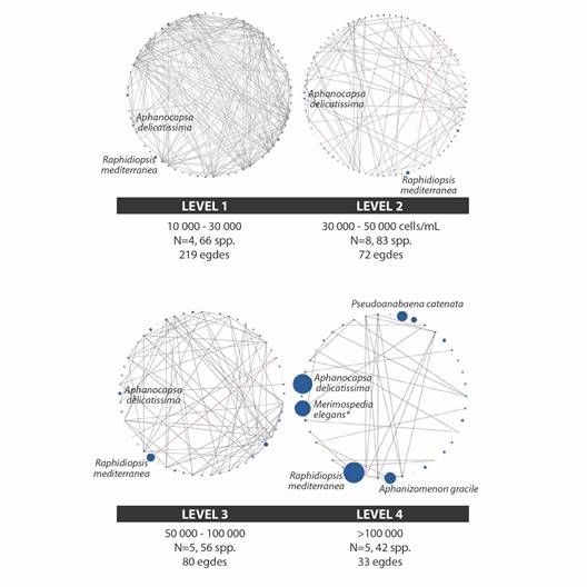
Fig. 3 Correlation abundances networks by level. Black edges represent positive correlations while red ones denote negative correlations. Circle sizes are proportional to specific abundances. Colors show groups: blue: Cyanobacteria, green: Chlorophyceae, yellow: Bacillariophyceae, turquoise: Euglenophyceae, dark brown: Dinophyceae, light brown: Ochrophyta, red: Xantophyta. * The dominant species (higher abundances) are highlighted in the figure. The black lines in the charts represent positive correlations, and the red lines represent negative correlations.
Discussion
Correlation abundance networks aid in understanding the relationships within the phytoplanktonic community and could be a powerful tool for monitoring cyanobacteria blooms.
The trophic state of the El Limón reservoir was predominantly mesotrophic throughout the period, which aligns with the overall state of reservoirs in Argentina (O’Farrell et al., 2019; Amé et al., 2003; Bazán et al., 2005). Nutrient concentrations, mainly dissolved nitrogen and soluble reactive phosphorus, showed no significant differences over the analyzed cycle or between proposed classification levels. Based on these results, we can infer that the differences in the intensity of the blooms may be mostly promoted by temperature, which did show differences between levels, and helped by the biological interactions of the bloom-forming species with the rest of the community.
Cyanobacterial blooms have been recurrent in the El Limón reservoir during the study period, highlighting the issue and rendering the reservoir a risk-prone environment due to its use for water consumption. Over time, these blooms became increasingly intense. Previous studies conducted in tropical reservoirs exhibit similarities to the results of the present work, with a predominant representation of Aph. gracile, R. raciborskii, M. flos-aquae, Pseudanabaena spp., R. mediterranea, and Dolichospermum spp. (Harke et al., 2016). These genera have been frequently observed in Argentina as well as in reservoirs in the central and Southern regions of Brazil (Echenique et al., 2006; Salusso & Moraña; 2018), despite existing morphohydrological differences between them (Moschini et al., 2009; Sant’Anna et al., 2007). These similarities in cyanobacterial community components based on climatic conditions might indicate a geographic spread of blooms at a regional level (Bittencourt-Oliveira et al., 2014), especially of invasive species that have expanded their current dispersal range, such as Cylindrospermopsis (Cires & Ballot, 2016).
The analysis of correlation abundance networks at different bloom intensities allows us to delve into the effect of blooms on the phytoplankton community and to formulate biological hypotheses of bloom-forming algae and cyanobacteria. Despite decreasing species richness during intense blooms, the relationships among phytoplankton species also declined. But what are the possible ecological implications of correlated abundances? positively correlated abundances could be associated with co-aggregation, cross-feeding, co-colonization, niche overlap, cooperation, or facilitation, while negative relationships could be linked to competition or amensalism (Deng et al., 2012; Faust & Raes, 2012). In the reservoir, we predominantly observed positive correlations, which might indicate the lack of net competition for resources. The prevalence of positive correlations could imply that all species respond similarly to external stimuli, such as environmental factors, thus their population growth is constrained by the same parameters. Given the predominantly mesotrophic to eutrophic state of the reservoir, it can be assumed that macronutrient requirements (N and P) were more than fulfilled during all sampling dates. The overwhelming positive correlations across all levels could be also explained by the possible cooperation leading to coupling and positive feedback among phytoplankton species, enhancing overall metabolic efficiency within the community (Coyte et al., 2015).
Remarkably, predominant cyanobacterial species exhibited limited interconnectivity in the correlated abundance networks observed at low bloom levels; appearing to have maintained a degree of isolation from the broader community in the most severe bloom, they were all of them practically completely disconnected. For example, Raphidiopsis mediterranea in level 3 was correlated only with 2 species, Crucigenia tetrapedia and Cyclotella sp., while in level 4, it was correlated only with Scenedesmus spinosus. Given the low number of correlations in these levels, these correlations might well be random and lack biological significance. The fact that the primary bloom-forming species becomes completely disconnected from the phytoplankton network could indicate its capacity to dominate the phytoplankton network (Lozano, 2022). Conversely, strongly correlated species in a network respond similarly to environmental conditions, probably limiting the capability of each one to dominate. The disconnection from the community could increase the probability of successful bloom, as it remains “independent” of the network. Abundance correlation networks could be useful in identifying bloom-forming species, as their ecological behavior is key to their dominance. This study is exploratory, seeking new applications for the tool, so it is advisable to continue refining it and use larger sample sizes.
Ethical statement: the authors declare that they all agree with this publication and made significant contributions; that there is no conflict of interest of any kind; and that we followed all pertinent ethical and legal procedures and requirements. All financial sources are fully and clearly stated in the acknowledgments section. A signed document has been filed in the journal archives.

