


 English (pdf)
 Article in xml format
 Article references
 Send this article by e-mail
 Cited by SciELO
  Similars in
SciELO
Similars in
SciELO  uBio
uBio 
 Permalink
Introduction
Aquatic macroinvertebrates are widely used to understand general biological distributional patterns and are also used extensively as indicators of the biological quality of freshwater ecosystems (Resh et al., 1995). Chironomidae (Diptera) is the most widespread of aquatic insect families (Ferrington, 2008) and is the most abundant insect group in aquatic ecosystems (Armitage et al., 1995; Shadrin et al., 2017; Shadrin et al., 2019). Their immature stages (larva and pupa) are very important in aquatic trophic webs; constituting a considerable part of the diet of other invertebrates, fishes, amphibians and birds (Armitage et al., 1995). In addition, different taxonomic levels of Chironomidae (subfamily, genus or species) have been considered good indicators of water quality for biomonitoring (Molineri et al., 2020). However, due to taxonomic difficulties, chironomids are often only identified at family level in broad spatial scale studies and biomonitoring programs (Lencioni et al., 2018; Rossaro et al., 2022).
Many studies carried out in the Holartic region have recorded variation in chironomid larval assemblages along spatial and altitudinal gradients (Lindergaard & Brodensen, 1995; Rossaro et al., 2006). These studies reported that Orthocladiinae, Diamesinae, and Prodiamesinae are the predominant taxa in mountain streams while Chironominae (especially, Chironomini) increase toward the lowlands. Water temperature and current regime were proposed to be the main factors related to the distributional patterns observed in these assemblages (Eggermont & Heiri, 2012; Rundle et al., 2007). In Europe, several studies that have included data from Chironomidae at genus level, found that the composition was concordant with river classifications, such as geomorphological division (Schöll & Haybach, 2004), ecotypes (Puntí et al., 2007; Puntí et al., 2009), or ecoregions (Plóciennik & Karaouzas, 2014). However, the differences among assemblages were small in some cases (Puntí et al., 2007), indicating an important overlap between chironomid assemblages and suggesting that a top-down classification of streams (using ecotypes) does not necessarily imply exclusive assemblages of chironomids.
Some studies of Chironomidae from the Neotropical regions have reported similar distributional patterns along altitudinal gradients. Orthocladiinae, Diamesinae and Podonominae are more frequent in high elevation streams, while Chironominae are dominant in lowland rivers (Acosta & Prat, 2010; Medina et al., 2008; Principe et al., 2008; Rodríguez Garay et al., 2020; Scheibler et al., 2014; Tejerina & Malizia, 2012; Tejerina & Molineri, 2007; Villamarin et al., 2021; Zanotto-Arpellino et al., 2015). Chironomidae studies from neotropical lowlands streams and rivers in semiarid zones such as those of the Western Chaco dry forest, are still scarce. Nevertheless, recent studies that analyzed benthic macroinvertebrates distribution in rivers of the Western Chaco ecoregion revealed that chironomids are the most abundant invertebrate group (Leiva et al., 2020; Pero et al., 2019).
In addition, it is also important to know the seasonal variations of freshwater ecosystems features across contrasting climatic but contiguous regions, mainly because of the uncertain challenges of climate change (Tonkin et al., 2019) and for the inference of reference conditions for the bioassessment (Hawkins et al., 2010). Some studies associated seasonal disturbances in streams, such as spates and floods, as important features structuring Chironomidae assemblages (Langton & Casas, 1998; Rossaro et al., 2006). The relative abundance of Chironomidae subfamilies also showed temporal variation in neotropical streams, such as those of Yungas forest. For example, Orthocladiinae was better represented during low water period whereas Chironominae was more abundant in high-water period (Tejerina & Malizia, 2012). Nonetheless, Acosta and Prat (2010) found that in both the dry and rainy seasons, the subfamily Orthocladiinae was dominant, surpassing 70 % of the total of Chironomidae in high elevation streams of Andean region of Peru.
It is important to know the distributional variations of these aquatic insects in reference conditions along the landscape to improve water quality bioassessments (Nicasio & Juen, 2015) and extend our knowledge about how climatic and ecoregional gradients influence the distribution and function of the freshwater neotropical biota. Therefore, our main goal was to explore the vertical and spatial distribution of chironomids in Northwestern Argentina, expanding the study area in the Yungas Forest with respect to Tejerina and Malizia (2012) and including a comparative analysis with rivers of the little-explored and highly threatened Western Chaco ecoregion (which represent the first specific study on chironomids for this region). Hence, we aimed to answer: (1) How do the composition and structure of Chironomidae assemblages (genus and subfamilies) vary between Yungas and Western Chaco ecoregions and among mountains, foothills and lowlands in Northwestern Argentina? (2) How do composition and structure of Chironomidae vary between hydrological seasons (low and high-water periods)? (3) How is Chironomidae distribution related to the environmental features of the studied rivers?
Materials and methods
Study Area: The study area is located between (26°-28° S & 66°-64° W) and covers approximately 20 000 km2 including most of Tucumán province and its limits with Santiago del Estero province in Northwestern Argentina (Fig. 1). In this study, we sampled reaches of fluvial channels located in two different ecoregions: Yungas subtropical cloud forest and Western Chaco dry forest (Brown & Pacheco, 2006).
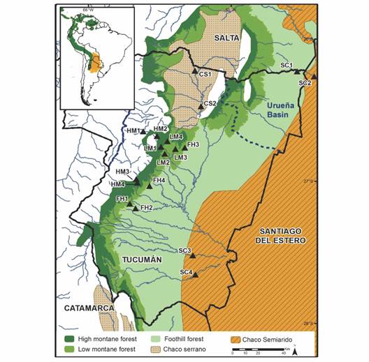
Fig. 1 Study area and sampling site locations. Sites codes: HM = high montane; LM = low montane; FH = foothill forest; CS = Chaco Serrano; SC = Semiarid Chaco.
The Yungas subtropical cloud forest or Yungas forest is a narrow belt of mountain rainforest, ranging from 400 to over 3 000 m.a.s.l. (Brown, 2000). The climate is warm and humid, with annual average temperatures ranging from 14 to 26 °C and rainfall from 1 000 to 2 500 mm (Brown et al., 2001). The Yungas forest is stratified into 3 vegetation belts. In general, Yungas altitudinal levels are not considered sub-ecoregion units, but in this study, we evaluated them as differentiated units within the Yungas forest because each altitudinal level presents particular climatic features and floristic composition (Brown & Pacheco, 2006). The high montane forest (1 500-3 000 m.a.s.l.) contains monospecific tree stands that are usually either Alnus acuminata (Kunth) or Podocarpus parlatorei (Pilg.). Annual rainfall reaches 1 000 mm. The low montane forest (700-1 500 m.a.s.l.) has the most diverse vegetation, with many evergreen species, and is dominated by Cinnamomum porphyrium (Griseb.) Kosterm. and Blepharocalyx salicifolius (Kunth) O. Berg. The low montane forest also has the highest precipitation (2 000 mm annual) and least seasonal hydrological regime. The foothill forest (400-700 m a.s.l.) contains deciduous trees and is dominated by Tipuana tipu (Benth.) Kuntze and Enterolobium contortisiliquum (Vell.) Morong. The annual rainfall varies between 1 000-1 500 mm during the wet season, and the 6-month dry season (£ 50 mm rainfall) extends from June to November (Brown et al., 2001).
The Western Chaco ecoregion is a vast sedimentary fluvial plain formed by the streams and rivers that run Northwest to Southeast and includes parts of Northwestern Argentina, Southeastern Bolivia, Northwestern Paraguay, and Southwestern Brazil (Great South American Chaco). The headwaters are located in the mountains, outside the region to the West, and they transport great quantities of sediments into the region. Mean annual temperatures range between 19 and 24 °C. Annual rainfall varies between 400 and 900 mm, with most precipitation falling in the summer and little falling in the winter (Minneti, 1999). The vegetation is composed of dry forests and segregated grasslands. This ecoregion is classified into three sub-ecoregions: Arid Chaco, Semiarid Chaco, and Chaco Serrano (Brown & Pacheco, 2006). Only the last two are represented in the study area. The Chaco Serrano is part of the Western border of the ecoregion and is characterized by low mountain topography. The Semiarid Chaco occupies the greater portion of the ecoregion and is a continuous xerophytic and semi-deciduous forest.
Within the study area, five river types (montane forest (I), foothill forest (II), Chaco Serrano (III), Semiarid Chaco pebble rivers (IV), Semiarid Chaco sand rivers (V)) have been identified and included in three large groups: Mountains, Foothills, and Lowlands (Plains) rivers (Pero et al., 2020). In the classification of Pero et al. (2020), a combination of ecoregions and topography was the main criteria to define river types and the physical variables as altitude, grain size, water temperature and turbidity were key parameters to develop the river typology.
Survey design and methods: We studied 18 sites (Fig. 1). Sites were distributed across ecoregions and sub-ecoregions as follows: 12 in the Yungas subtropical cloud forest (4 in high montane (HM), 4 in low montane (LM), and 4 in foothill forests (FH)), and 6 in the Western Chaco (2 in Chaco Serrano (CS) and 4 in Semiarid Chaco (SC)). Each site consisted of a stream reach ~100 m long. We chose sites that were minimally disturbed, without industrial impact, and with native riparian vegetation at least 100 m wide.
Data from 13 of the 18 sites (HM3, HM4, LM4, FH1, FH2, FH3, FH4, CS1, CS2, SC1, SC2, SC3 and SC4) were collected between 2014 and 2018 by the authors. Data for the 5 other sites (HM1, HM2, LM1, LM2, LM3) were obtained from the IBN (Neotropical Biodiversity Institute, National Council of Technological and Scientific Research - National University of Tucumán) database and are published elsewhere (Tejerina & Malizia, 2012). The IBN sites were sampled between 2005 and 2007 following the same collection procedures. Climate conditions were similar during these 2 periods according to local climate databases, and both periods corresponded to the ENSO phase of El Niño according to the Oceanic Niño Index (ONI) (http://www.cpc.noaa.gov/products/analysis_monitoring/ensostuff/ensoyears.shtml). In addition, previous studies in the region observed that macroinvertebrate assemblage composition and structure changes seasonally rather than annually (Mesa, 2012). All sites were sampled once at the end of the low-water period (October-December) and once at the end of the high-water period (March-June) for two years, with the exception of 2 sites that were sampled only during the low water period (FH3, SC3).
Chironomidae sampling: At each site we collected quantitative and qualitative samples. Three quantitative samples were collected with a Surber net (0.09 m2 area with a 300 µm mesh), and were subsequently pooled into a single, composite sample. We took these samples in fast-water habitat units (riffles or runs, sensu Hawkins et al., 1993) that were separated by 50 m along a longitudinal transect. The qualitative samples consisted of samples collected with a D-frame net (300 µm mesh), a kick-net (500 µm mesh), and by manual sampling. Manual sampling included directly picking specimens from boulders, cobbles, leaves, and algae. The qualitative sampling took approximately 30 minutes to cover all habitats. Riffles, pools, and marginal vegetation habitats were most common. All samples were preserved in ethanol 96º. Quantitative data were used to analyze abundance patterns, and the combined quantitative and qualitative data were used to analyze presence-absence data. We brought all samples to the lab after collection, where we processed and identified each entire sample. In the laboratory, chironomids larvae were sorted, counted and identified to morphospecies using a stereomicroscope with a 10X magnification (Rossaro et al., 2022). From each morphospecies, we chose those corresponding to the fourth stage larvae to make permanent microscope slides. Larvae were mounted complete (including head capsules and body) following the conventional method proposed by Epler (2001). Larvae were identified using a compound microscope with 40-100X magnification to genus level using taxonomic keys (Andersen et al., 2013; Epler, 1995; Epler, 2001; Merritt & Cummins, 1996; Trivino-Strixino & Strixino, 1995; Wiederholm, 1983) and other taxonomic works (Cranston & Krosch, 2011; Prat et al., 2017). The rest of the material that was not used to make permanent microscope slides was preserved in 75 % ethanol.
Environmental variables: We characterized the environmental setting at each site. We recorded elevation (m.a.s.l.) with a Garmin eTrex 20™ global positioning system (with an accuracy of 3 meters). Channel width (m), discharge (m3/s), water temperature (°C), pH, and conductivity (µS/cm) were recorded at every visit. We estimated discharge by measuring cross-sectional area, taking depth measurements every 25 cm (for streams ≤ 11 m wide) or 1 m (for rivers ≥ 11 m wide) along 1 cross-sectional transect across the channel, and measuring velocity with a velocity meter at 2/3 the depth at each point (Global Water Flow Probe FP111). Physicochemical variables were measured with a Horiba™ multi-probe water quality checker U-50 series.
Data analyses: All statistical analyzes and graphs were produced via the R platform (version 3.6.1, R Core Team, 2019) and via Microsoft Office Excel 2007.
Rank-abundance curves: We used rank-abundance (RA) curves (also known as dominance-diversity curves) to compare how assemblage structure varied across the different ecoregions, river types, and seasons. RA curves, in combination with species identity, can provide insight into specific patterns of species diversity, dominance, rarity, and composition (e.g., Pero et al., 2019). We used these analyses to complement the multivariate analyses and allow more detailed observations of compositional and structural differences among assemblages. Groups of dominant taxa, and taxa that occurred exclusively in each ecoregion and sub-ecoregion were identified. The 3 most abundant taxa at each site were considered the dominant taxa for each ecoregion and sub-ecoregion.
Dissimilarity: We used the Sørensen and the Positive Matching indices (PMI, Dos Santos & Deutsch, 2010) to analyze the presence-absence data. We used the Bray-Curtis and Dissim indices (Nieto et al., 2017) to estimate compositional dissimilarity between Chironomidae assemblages based on our abundance data. The PMI can vary between 0 and 1 and represents the mean proportion of ''positive matches'' relative to the complete list of taxa that could occur at a site. The PMI covers the range of richness encompassed by the two lists - i.e., the smaller and longer ones. Hence, if 2 lists of different lengths are compared, for example of 10 and 100 specimens, and the PMI is 0.3, that result indicates that the 2 lists share 30 % of taxa, on average, given the list sizes range from the smaller to the longer one (Dos Santos & Deutsch, 2010). In contrast, Euclidean and Bray-Curtis distances are 2 dissimilarity indexes that are frequently used in ecological analyses (Nollet & De Gelder, 2014). However, both of these indices are strongly influenced by dominant species and are only weakly affected by rare species (Valentin, 2012) and are therefore not as useful when there are gradual changes in composition along a gradient. The Dissim index can be used when the observed taxa are assumed to have been sampled from a common regional pool of species. The Dissim Index assesses whether assemblages are similar based on both the taxa present and their abundance. Thus, 2 sites would be considered more similar whether they grouped consistently near each other after successive orderings of sites by increasing values of consecutive taxa abundance (Nieto et al., 2017).
We used multivariate analyses to determine if differences in assemblage composition among sites were associated with regional classifications. We used Nonmetric Multidimensional Scaling (NMDS) based on dissimilarity values obtained from presence-absence and abundance data to illustrate whether the positions of sites in taxa space were concordant with ecoregional and typological classifications. We interpreted how discrete the ecoregions and river types were by drawing a convex polygon around each group of river types on the NMDS plot.
It is well known that benthic macroinvertebrate assemblages can vary markedly with season (Poff & Ward, 1989). We therefore separated the data by low and high waters periods to test whether the differences among ecoregions, sub-ecoregions and river types were greater than the seasonal differences within each site.
For the description of the structure and composition of Chironomidae subfamilies, we estimated the relative abundance of each subfamily for each ecoregion and river type.
Envfit analysis: To assess the set of environmental variables that best correlate with biological ordinations, vectors (selected environmental variables) were fitted to the existing NMDS plots of sample dissimilarities using the function ''envfit'' (from R package vegan). The envfit scales these vectors based on their correlation coefficient, and the resulting plot allows to quickly identify the most important variable gradients represented by the NMDS plot (Clarke & Ainsworth, 1993).
Results
Composition and structure of Chironomidae larvae assemblages at subfamily level: We collected 11 724 Chironomidae larvae across sampling sites (without counting data from the IBN database). In the total dataset, we identified 34 genera belonging to five subfamilies. The subfamilies Chironominae and Orthocladiinae showed the highest abundance (47.3 % and 46.1 % respectively), Tanypodinae constituted 5.7 %, while Diamesinae and Podonominae showed the lowest abundance (0.85 and 0.01 % respectively). Genera richness was similar among Orthocladiinae, Chironominae and Tanypodinae (11, 10 and 10 respectively), whereas Podonominae comprised 2 genera and Diamesinae only 1 genus.
The relative abundance of the five Chironomidae subfamilies varied across the ecoregions. Orthocladiinae was more abundant in Yungas forest and high elevation sites and decreased downstream, but including Chaco Serrano sites. Chironominae showed the opposite pattern, being dominant in Semiarid Chaco and lower elevation sites. Diamesinae had a relative low abundance, peaking in the highest Yungas vegetation level (between 2 170 and 1 200 m.a.s.l.) and decreasing toward foothill forest (between 700 and 400 m.a.s.l.). This subfamily was absent in the Chaco ecoregion. Podonominae were recorded in one site at high montane forest and with very low abundance. Tanypodinae had low abundance in most of the sites but had a peak of 12 % in Semiarid Chaco sites.
Composition and structure of Chironomidae larvae assemblages at genus level: Cricotopus was the most abundant taxa in all Yungas regions and at the two hydrological seasons. Some genera were recorded exclusively in Yungas forest streams. Barbadocladius and Genus 10 were only present in high montane forest and Genus X was present in high and low montane forest, Parametriocnemus was found in all subecoregions from Yungas forest but was not recorded in Western Chaco. The genera Parochlus and Podonomus from Podonominae subfamily were only recorded at high montane forest. The genera Apsectrotanypus and Larsia (Subfamily Tanypodinae) and Paraheptagyia (Subfamily Diamesinae) were only present in rivers from high and low montane forests. Within streams and rivers from Western Chaco, the more abundant genera were Onconeura (Orthocladiinae), Rheotanytarsus and Polypedilum (Chironominae). In addition, some genera were found exclusively in Semiarid Chaco rivers, mainly from the subfamily Chironominae: Cryptochironomus, Harnischia 1, Robackia, Saetheria; and Tanypodinae: Procladius, Nilotanypus and Clinotanypus. The genera Lopescladius, Onconeura (Orthocladiinae), Rheotanytarsus, Tanytarsus and Polypedilum (Chironominae) were present in all ecoregions and river types.
The results included new records of some genera for North-western Argentinean provinces. Robackia, Cryptochironomus, Saetheria (Chironominae), possibly Denopelopia, Labrundinia, Tanypus and Procladius (Tanypodinae) were recorded for the first time for Tucumán province; Clinotanypus and Thienemannimyia (Tanypodinae) for Tucumán and Santiago del Estero provinces; Pseudochironomus (Chironominae) and Nilotanypus (Tanypodinae) for Santiago del Estero.
Dissimilarity: The overall structure of the Chironomidae assemblages was concordant with the ecoregional and river typology classifications based on either presence-absence or abundance datasets (Fig. 2). NMDS axis 1 from both abundance and presence-absence analyses segregated two groups: one composed of the Yungas sites, which included river types I and II, and another composed of Western Chaco sites, which included river types III, IV and V. The seasonal differences among sites were much lower than the ecoregional and typological dissimilarities.
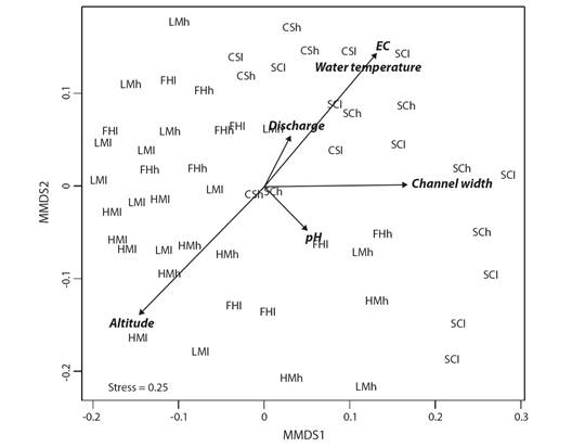
Fig. 2 Non-metric multidimensional scaling (NMDS) plot of Chironomidae samples dissimilarity at the genus level using abundance data (Dissim index) with best correlated environmental variables from Envfit analysis. HM = high montane; LM = low montane; FH = foothill forest; CS = Chaco Serrano; SC = Semiarid Chaco. l = low waters; h = high waters.
Correlations among abiotic and biotic ordinations: According to the envfit analyses, the axes of the NMDS plots were significantly correlated with some abiotic features (Table 1) of the rivers (Table 2). Finally, the grouping of the Yungas assemblages, mainly from high and low montane forest (river type I) was more related to higher elevations, while Western Chaco assemblages (river types III, IV and V) were strongly related to high values of water temperature, conductivity and channel width (Fig. 2). Foothills forest assemblages (river types II) had an intermediate position in the observed biotic-abiotic gradient.
Table 1 Associations between environmental variables (vectors) and the non-metric multidimensional scaling (NMDS) ordination plot of Chironomidae samples dissimilarity at the genus level using abundance data (Dissim index) (dimensions 1 and 2) using the envfit function (R package vegan)
| Vectors | Dimension 1 | Dimension 2 | R2 | P |
| Altitude | -0.73 | -0.69 | 0.43 | 0.001 |
| Discharge | 0.49 | 0.87 | 0.04 | 0.319 |
| Channel width | 0.99 | 0.01 | 0.29 | 0.001 |
| Water temperature | 0.68 | 0.73 | 0.28 | 0.001 |
| Electric Conductivity (EC) | 0.67 | 0.74 | 0.40 | 0.001 |
| pH | 0.72 | -0.69 | 0.05 | 0.253 |
Table 2 Environmental variables measured at study sites (mean values)
| Elevation (m.a.s.l.) | Discharge (m3 s -1) | Channel width (m) | Water temperature (°C) | Conductivity (µS/cm) | pH | |
| HM1 | 2 170 | 0.57 | 8.9 | 12.7 | 57.0 | 7.0 |
| HM2 | 1 300 | 0.14 | 1.9 | 18.7 | 126 | 6.7 |
| HM3 | 1 622 | 0.36 | 3.6 | 10.6 | 78.5 | 8.1 |
| HM4 | 1 394 | 0.09 | 1.7 | 12.7 | 68.8 | 7.5 |
| LM1 | 925 | 2.04 | 7.1 | 17.1 | 124 | 6.6 |
| LM2 | 680 | 0.54 | 8.9 | 21.0 | 447 | 7.5 |
| LM3 | 860 | 0.12 | 3.7 | 18.7 | 287 | 7.0 |
| LM4 | 1 126 | 0.04 | 1.3 | 16.9 | 226 | 8.3 |
| FH1 | 711 | 0.93 | 7.1 | 19.1 | 52.5 | 7.2 |
| FH2 | 543 | 5.26 | 23 | 16.2 | 86.7 | 7.6 |
| FH3 | 713 | 0.03 | 1.4 | 18.8 | 246 | 8.3 |
| FH4 | 590 | 0.22 | 6.0 | 14.9 | 70.5 | 7.9 |
| CS1 | 761 | 3.71 | 21 | 19.9 | 556 | 7.5 |
| CS2 | 649 | 7.57 | 28 | 18.5 | 737 | 7.8 |
| SC1 | 429 | 1.58 | 9.9 | 22.2 | 2 370 | 7.7 |
| SC2 | 398 | 1.37 | 7.8 | 25.4 | 2 576 | 7.7 |
| SC3 | 307 | 5.53 | 74 | 28.5 | 504 | 8.4 |
| SC4 | 291 | 8.12 | 38 | 20.2 | 848 | 8.1 |
Discussion
We found that Chironomidae assemblages' distribution corresponded with the landscape analysed units, both ecoregions and river types. However, the ecoregional classification better fitted chironomid distribution. In addition, the composition of Chironomidae assemblages at subfamily level along the altitudinal gradient studied was very similar to the ones described in other studies (Lindergaard & Brodersen, 1995; Principe et al., 2008; Tejerina & Malizia, 2012). Orthocladiinae was dominant at higher elevation sites and Chironominae was more abundant at lowland rivers. Chironomidae distribution was related to the variations of environmental features along the landscape, as was reported in several previous studies in other regions (Acosta & Prat, 2010; Rodríguez Garay et al., 2020; Villamarín et al., 2021), mainly elevation, water temperature and conductivity. Seasonal differences in Chironomidae assemblages were weaker than ecoregional ones, as it was observed for other invertebrate groups in the study area (Pero et al., 2019; Pero et al., 2020).
Our results provide information that helps to understand how different classification systems reflect the natural variability that exists along the landscape and altitudinal gradients. The Chironomidae assemblages corresponded with the ecoregional scheme in a broad spatial scale, but typology also allowed subdividing them by finer river types. Similarly, other studies that tested river typologies distinguished groups of Chironomidae assemblages based on river types (Plóciennik & Karaouzas, 2014; Puntí et al., 2009; Schöll & Haybach, 2004). However, differences among river types were not strong, indicating certain overlap between chironomid assemblages with the established ecotypes, as it was reported by Puntí et al. (2007) for Mediterranean streams in Spain and also suggesting that a top-down classification of streams (using ecotypes) does not necessarily imply exclusive assemblages of chironomids.
The segregation of Chironomidae assemblages among regions and river types was most strongly related to broad spatial scale variables, such as altitude, and associated physiochemical variables, such as water temperature or conductivity. As it was recorded in previous studies in neotropical streams (Acosta & Prat, 2010; Tejerina & Malizia, 2012), the presence of taxa from the subfamilies Podonominae and Diamesinae, and the dominance of Orthocladiinae was related to high elevation sites with low water temperature and conductivity. The dominance of Chironominae in lowland rivers with higher values of water temperature and conductivity observed in our study was also evidenced in other neotropical regions (Leiva et al., 2020). In addition, we found that in certain lowland river types, with higher levels of conductivity, the subfamily Tanypodinae was more important, in terms of its relative abundance, than in the other sub-ecoregions and river types. For example, the genus Procladius, belonging to that subfamily, was very abundant. This genus was found to be resistant and abundant in other areas of high salinity (Wolf et al., 2009). These results showed that local environmental features could also influence Chironomidae assemblage composition.
The findings of our study support the proposal that topography in conjunction with biogeographical history of assemblages could act synergistically as drivers of assemblage composition in the South American geographical context (Pero et al., 2019). In our study area, topography varied throughout the South American biogeographical transition zone that separates the High Andean (including the higher areas of Yungas) and the Amazon (including lower areas of Yungas and Chaco) biogeographical regions (Morrone, 2014). In addition, Dos Santos et al. (2018) revealed that the distribution of Ephemeroptera assemblages was strongly influenced by the segregation of ''cool adapted'' taxa all across and toward the East and Southeast of the Andes, and ''warm adapted'' taxa to the foothills and lowlands located toward the west and Northwest of the Andes. Similarly, Chironomidae assemblages could also be influenced by both the biogeographical and ecological South American context. Finer levels of taxonomical identifications could add more information about biogeographical patterns (Rossaro et al., 2022). For example, the genus Cricotopus in the Andes is quite complex, and many taxa were recently considered as subgenera of this group. According to recent studies, Oliveiriella (recorded in many sites of our study area, Tejerina & Paggi, 2009) is not a genus but a subgenus of Cricotopus (Andersen et al., 2013; Prat et al., 2017). In addition, the diversity of Rheotanytarsus (Chironominae) is very high in Latin America with many species to be described (Dantas et al., 2020), and this is an additional problem. Hence, further studies about taxonomical and distributional aspects of Chironomidae are still necessary to better understand their ecology and biogeography in the neotropical region.
Seasonal differences in Chironomidae assemblages were lower than ecoregional ones, which showed that temporal variations would not affect the regional classifications tested. No exclusive assemblages were distinguished or associated to any hydrological season compared (low or high water period), in contrast to the observed for chironomid summer samples in Mediterranean streams (Puntí et al., 2007). Similarly, Acosta and Prat (2010) found that in both the dry and rainy seasons, the subfamily Orthocladiinae was dominant in high elevation streams of Andean region. Nevertheless, we found greater differences in chironomids abundance rather than in their genera composition between seasons, generally showing the lowest abundance during high water periods when spates and floods are frequent, as was reported by other studies (Tejerina & Malizia, 2012).
The information gathered in our study about the assemblages of Chironomidae allows us to better understand the relationships between the landscape and the distribution of biota from the perspective of a biological group little studied in the region. In addition, our results support the use of ecoregions and river typologies to improve our ability to establish the reference conditions for South American fluvial ecosystems. Finally, our findings expand our knowledge about the ecology and distribution of neotropical freshwater chironomid assemblages, providing data from little-explored and highly threatened ecoregions.
Ethical statement: the authors declare that they all agree with this publication and made significant contributions; that there is no conflict of interest of any kind; and that we followed all pertinent ethical and legal procedures and requirements. All financial sources are fully and clearly stated in the acknowledgements section. A signed document has been filed in the journal archives.

