


 Inglés (pdf)
 Articulo en XML
 Referencias del artículo
 Enviar articulo por email
 Citado por SciELO
  Similares en
SciELO
Similares en
SciELO  uBio
uBio 
 Permalink
Introduction
In the management of native forests, forest inventory is an essential procedure for forest planning. According to de Araujo (2006), in areas where forest management is required, forest inventory is a key to understanding the composition and structure of the forest, through the gathering of information from natural regeneration to the adult stage; it allows to determine the potential and aptitude for the management of the area.
Forest inventory is responsible for quantifying available resources, assessing their quality, and providing information that supports the decision-making process to implement a management system (Farias, 2012). According to the same author, this activity also aims to monitor managed species to obtain information about possible impacts on the regeneration of such species and the remaining fauna and flora.
Forest inventories play several roles in the management of native forests. They provide information about the stock of non-timber species (Farias, 2012), forest carbon (Higuchi et al., 2004; Vianna et al., 2010), and forest structure (Cavalcanti et al., 2009; Cavalcanti et al., 2011; Ubialli et al., 2009), among other purposes. In the Amazon forest, according to de Oliveira et al. (2014), inventories are mainly used for volume estimation, as a tool to evaluate the technical and economic feasibility of forest management plans in private properties.
Inventories performed in the Amazon rainforest adopt several methodologies (Silva, 1980; Silva & Lopes, 1984; Silva et al., 2005), besides the network of permanent plots as Rainfor - Amazon Forest Inventory Network and TmFO - Tropical Managed Forests Observatory, especially with the emphasis on the size and shape of the plot and also in the definition of the minimum inclusion diameter, which ends up being a problem. This variation in the size and shape of the plots as well as the sampling intensity can lead to uncertainties in forest inventory (de Oliveira et al., 2014).
In this sense, absence of standardization in forest inventory can generate certain consequences. They refer to information loss, low accuracy, and inconsistent measurement standards which compromise the use of the collected information in national or international networks and processing software. Thus, standardization of the methods would allow the researcher to benefit from common expertise, enhance research activities, favor the valorization and dissemination of results, and optimize the available resources.
Thus, when considering the hypothesis that plot with 10 000 m² of área are the better to realize the forest inventory diagnostics in amazonia Pantropical, we suggested other three variations in this size (2 500, 5 000 and 7 500 m²) compared with the 10 000 m² size, to provide adequate precision for the estimation of dendrometric parameters and diversity in an area of Mixed Submontane Forest, in the legal Brazilian Amazon region, Mato Grosso State.
Materials and methods
Study area: This study was conducted at the São Nicolau farm, owned by the company ONF Brazil. The farm is located in the legal Amazon region (ME, 2019), Cotriguaçu city, northwest of the Mato Grosso State, around the coordinates 58.24 S and 9.84 W (Fig. 1). The farm has a total area of 10 287 ha, which 7 500 ha is of native forest. Of these 7 500 ha of native forest, 1 800 ha have been used as a Private Reserve of Natural Heritage (RPPN Peugeot ONF), while the remnant of the native forest area was used for sustainable timber production.

The property is located in a region with an “A'' type climate, according to the Köppen method (Alvares et al., 2013). The region has average annual temperatures between 25 °C and 27 °C, an average annual rainfall of 2 500 mm, and relative humidity of 85 %.
The original forest type of the area under study, according to MME (1982), comprises the Tropical Open Rainforest typology, sub-montane formation with Palm trees. Its understory is quite dense, mainly due to the regeneration of palm trees. The region of the Open Ombrophyla Rainforest is called the “transition zone'' between the Amazon and the rest of the country.
Experimental design: The study was conducted in the Annual Production Unit 1 (UPA 1) of the Forest Management Plan of Fazenda São Nicolau, with 227 ha of area. Using QGIS (QGIS Development Team, 2018), a grid of size 100 m x 100 m was allocated throughout the study area. After that, the first plot was randomly chosen and the subsequent five were systematically defined, with a six sample plot allocated in this study area (Fig. 2).

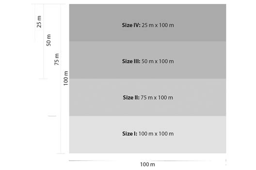
After the selection and installation of plots, they were divided into four subplots of 2 500 m² each, which allowed the definition of a spatial gradient of 2 500 m², 5 000 m², 7 500 m², and 10 000 m² across the dimensions of 25 m x 100 m, 50 m x 100 m, 75 m x 100 m and 100 m x 100 m, respectively (Fig. 3). The design resulting from the divisions of the allocated plots had four plot sizes, each with six repetitions, in which the variables of interest were analyzed. The number of samples in the study follow the requirements established by Decree 2152/14 of the Secretary of State for the Environment for the State of Mato Grosso, Brazil.
Data collection: Trees with diameters at breast height (DBH) ≥ 20 cm (Silva & Lopes, 1984) were measured and identified within the plots. From the trees not identified in loco, vegetative material was collected, pressed, and dried in an oven with forced ventilation at 60 °C for 48 hours, according to the herborization methodology indicated by the Technical Manual of Brazilian Vegetation (ME, 2012). The material for the identification of these species was then sent to the Herbarium IAN - EMBRAPA, in Belém, Para State, Brazil.
Metrics calculated: Initially, the floristic similarity between the different plot sizes was calculated, using the Jaccard Index (Equation 1), according to Magurran (1988).
 (1)
(1)
where: SJ = Jaccard similarity index; a = total number of species present in sample “a''; b = total number of species present in sample “b''; c = total number of species common to samples “a'' and “b''.
The diversity was obtained as proposed by Magurran (1988), by Shannon-Weaver Index (Equation 2).
 (2)
(2)
in which: H' = Shannon-Weaver diversity index; ni = number of individuals of the i-th species in the sample; N = total number of individuals in the sample; ln = Napierian logarithm (base e).
The Shannon's indexes were compared by Hutcheson's Test with 5 % of significance (Hugo & David, 2021; Hutcheson, 1970; Magurran, 1988).
The horizontal structure of the vegetation was evaluated through tree density (N.ha-1) and basal area (m².ha-1) calculated at plot level (Equation 3).
 (3)
(3)
where: AB = Basal Area (m²/ha); DBH = Diameter at Breast Height (cm); EF = Expansion Factor (EF = 4 for 2 500 m² plot size; 2 for 5 000 m² plot size; and 1.33 for 7 500 m² plot size).
Above Ground Biomass (AGB) was also estimated at the individual tree-level using the equation proposed by Chave et al. (2005) for humid forests (Equation 4). After obtaining this variable at the tree-level, the individual biomass of the trees per plot was summed and expanded to 1 hectare.
 (4)
(4)
where: AGB = Above Ground Biomass (kg/tree); DBH = Diameter at Breast Height (cm); ln = Napierian logarithm (base e); r = wood basic density.
The basic wood density values for each species to apply the Chave et al. (2005) equation were obtained from the Global Wood Density Database (Dryed) (Zanne, 2009). The confidence intervals were obtained for biomass (Mg.ha-1) and stocking density (n.ha-1).
The coefficient of variation was calculated to verify the dispersion of the data (Equation 5).
 (5)
(5)
where: CV = coefficient of variation (%); sd = standard deviation, = mean.
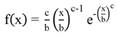
Subsequently, in all plot size conditions, the Weibull probability density function of two parameters and Gamma (Equation 6, Equation 7) were fitted. The AIC - Akaike Information Criteria was used to evaluate the best model to represent the data. (Equation 8). These functions were chosen because of the performance to describe curves with different shapes and flexibility.
 (6)
(6)
where: f(x) = density function of variable x; x = class center diameter; b = scale parameter; c = shape parameter.
 (7)
(7)
where: f(x) = density function of variable x; x = class center diameter; b = scale parameter; a = shape parameter;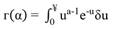 .
.
AIC = -2ln(mv)+2p (8)
where: ln = logaritimic of the value; mv = maximum likehood value; p = number of the parameters of the model evaluated.
Finally, dendrometric parameters were compared by the Dunnett's Test assumpting the 10 000 m² plot size with a control treatment. Further details can be obtained in Dunnett (1955) and Signorell et al. (2021).
All analyses were performed in R Software (R Core Team, 2019).
Results
Considering all the plots, a total of 877 individuals with DBH ≥ 20 cm were recorded in the forest inventory, with an average of 146 individuals per hectare. These individuals were distributed in 36 families and 119 species.
The richest species-diverse families were the following: Fabaceae with 34 species, Moraceae with 10, Malvaceae with 8, followed by Lecythidaceae, Meliaceae, and Sapotaceae, with 5 species each. Regarding the number of individuals per family, the most representative were as follows: Burseraceae (254), Moraceae (137), Fabaceae (108), and Sapotaceae (85), which represented 66.5 % of the total sampled individuals. More floristic informations can be obtained in Silveira (2019).
The different plot sizes generated values of Shannon-Weaver index (H') (Table 1), and they presented certain proximity among them. For the similarity, the Jaccard Index (Sj) (Table 1), it was observed that the largest plots presented higher index values than the smaller ones, when compared to the 10 000 m² plot (reference control plot size in this study).
Table 1 Shannon's s (H') and Jaccard' Index for each plot size
| Plot Size (m2) | H' | SJ* |
| 2 500 | 3.24 | 0.568 |
| 5 000 | 3.36 | 0.814 |
| 7 500 | 3.40 | 0.941 |
| 10 000 | 3.42 |
Note: The values of the Jaccard's Index were obtained from a comparison with the control plot - 10 000 m².
Table 2 shows the results obtained concerning mean diameter, mean population density (number of trees per hectare), basal area, and biomass, for the different plot sizes, extrapolated to one hectare. The main structural parameter that differed in the plots was biomass, where the smallest plot size showed a higher value compared with the other plot sizes, however without statistical difference as showed in Table 2.
Table 2 Mean parameters of dendrometric atributes for each plot size investigated in this study
| Variables | Plot Size | |||
| 2 500 m² | 5 000 m² | 7 500 m² | 10 000 m² | |
| DBH (cm)ns | 36.91 | 36.64 | 36.34 | 36.24 |
| Density (N ha-1)ns | 160.00 | 146.66 | 145.83 | 146.16 |
| Biomass (Mg ha-1)ns | 344.67 | 288.61 | 279.54 | 278.32 |
| Basal Area (m² ha-1)ns | 22.38 | 19.83 | 19.34 | 19.09 |
*ns = no signficance for the Dunnett test (a = 5 %). The control was the 10 000 m² plot size. DBH = diameter at breast height.
The statistics obtained for the density and biomass variables for the different plot sizes are shown in Table 3. The plot sizes that showed the lowest standard deviation and coefficient of variation were 10 000 m² and 7 500 m², respectively, which implies that these two sizes would result in a better statistical performance.
Although there were no significant differences in these results (Table 3). Fig. 4 shows that there is a tendency to reduce the coefficient of variation according to the increase in the plot area.
Table 3 Statistics for density and biomass variables for each plot size
| Variables | Estimators | Plot Size | |||
| 2 500 m² | 5 000 m² | 7 500 m² | 10 000 m² | ||
| Density (N.ha-1) | Mean | 146.19 | 146.41 | 146.47 | 146.11 |
| Standard Deviation | 18.55 | 13.61 | 10.65 | 9.09 | |
| CV (%) | 12.56 | 9.22 | 7.22 | 6.18 | |
| Lower C.I. | 109.08 | 119.19 | 125.16 | 127.92 | |
| Upper C.I. | 183.29 | 173.63 | 167.78 | 164.29 | |
| Biomass (Mg.ha-1) | Mean | 284.85 | 282.40 | 285.76 | 284.00 |
| Standard Deviation | 19.66 | 14.28 | 10.72 | 9.47 | |
| CV (%) | 6.46 | 4.76 | 3.53 | 3.18 | |
| Lower C.I. | 245.54 | 253.83 | 264.32 | 265.06 | |
| Upper C.I. | 324.17 | 310.96 | 307.20 | 302.94 | |
Note: CV - coefficient of variation; C.I. - confidence interval (95 %).

Through the AIC value, the best model was Gamma (Table 4), admitting that the 2 units it's sufficient to select one than other model (Burnham & Anderson, 2002). So, the Gamma model was used to represent the diametric distribution for all plot size.
In the analysis of the diametric structure obtained in the different plot sizes, the fitting of the Gamma function is show in histograms for each of the plot sizes, 2 500, 5 000 or 7 500 m², in comparison with the reference size, 10 000 m² (Fig. 4). The “inverted J'' behavior, characteristic of native forests, can be observed in all of them.
Table 4 AIC value for the models fitted
| Function | Plot size (m²) | AIC |
| Gamma | 2 500 | 1 992.832 |
| Weibull - 2p | 2 056.68 | |
| Gamma | 5 000 | 3 623.105 |
| Weibull - 2p | 3 750.546 | |
| Gamma | 7 500 | 5 386.31 |
| Weibull - 2p | 5 581.771 | |
| Gamma | 10 000 | 7 157.747 |
| Weibull - 2p | 7 419.148 |
It was also observed that the values of the parameters obtained, in the fitting of the diametric model (Table 5) for the different plot sizes, were very close to each other. These results contribute to the similarity across the curves observed in the Fig. 5.
Table 5 Gamma parameters for the four fitted models for each plot size
| Plot Size (m²) | Shape | Standard Error | Scale | Standard Error | p-value |
| 2 500 | 5.1849 | 0.4588 | 0.1396 | 0.0130 | < 0.0001 |
| 5 000 | 5.3388 | 0.3492 | 0.1464 | 0.0100 | < 0.0001 |
| 7 500 | 5.4341 | 0.2910 | 0.1504 | 0.0084 | < 0.0001 |
| 10 000 | 5.5578 | 0.2579 | 0.1542 | 0.0075 | < 0.0001 |

Discussion
The results obtained regarding the composition of families corroborate with other studies carried out in the Amazon region, such as those by Carim et al. (2013), Condé and Tonini (2013), and Pereira et al. (2011). In these studies, the number of individuals and the species richness contribute to the sovereignty of the inventoried families, which gives the physiognomic characteristics of the forest.
In the study conducted by Condé and Tonini (2013), the families with the highest number of species also represented a greater richness of individuals. Their result differs from the results obtained here since the Burseraceae family corresponds for 29 % of the total sampled individuals yet with the concentration of a single species, Protium autissimum. According to Amaral et al. (2000), abundance patterns are quite variable for species and families in general.
A study carried out in the Ecotonal Forest in the northern region of Mato Grosso, Ubialli et al. (2009) concluded that, according to the plot size, the distribution pattern of the species can change, and plots with larger dimensions up to 1 ha are indicated to obtain the real pattern of the spatial distribution of species in the area. To carry out phytosociological studies using a sampling intensity of 10 % and a random process, the estimates were accurate for the most economical and phytosociological important species, especially when using rectangular plots of 400 m² and 2 500 m². Ubialli et al. (2009) also commented that a plot size of 2 500 m² installed in a rectangular shape produces accurate estimates for phytosociological studies when considering the most important species groups from the economic and phytosociological point of view, regardless of the sampling process, but with a sampling intensity of 10 %.
The choice of the size of the sampling units in those cases in which the prediction of the parameters is not compromised by the reduction of the plot size can be made due to the operationality of the location and implantation. In this case, smaller units are advisable when time is a constraint, as suggested by Péllico Netto and Brena (1997).
The Shannon diversity index (H') of the different plot sizes was higher than 3.11, which according to Saporreti Jr. et al. (2003), indicates well-preserved area. Based on this criterion, the sampled forest can be characterized as a well-preserved area.
In all the different plot sizes, a similar assessment of the forest community diversity was obtained. This same index was higher when compared to savanna area in Brazil (Finger & Finger, 2015; Guilherme et al., 2004; Rodrigues-Sousa et al., 2015), with values 4.03, 3.86 and 3.85, respectively. The difference could be explained by the minimum diameter measured, where in these three studies was 10 cm. However, same values for the Shannon index was obtained by Apgaua et al. (2014). The forest researched by the authors was Tropical Forest with a dry season. The value obtained was 3.6. According to Rodrigues-Sousa et al. (2015), the Shannon index, when evaluated for each indivudal, was 3.55 in Riparian Forest.
In the evaluation of similarity, by Jaccard index, the plots with the highest similarity were the ones with 5 000 and 7 500 m², and the one of 2 500 m² presented the lowest value compared with the standard plot size of 10 000 m². However, for all plot sizes, the Jaccard index was higher than 0.5, which, according to Kent and Coker (1992), indicates high similarity.
The mean values of the basal area for the category DBH ≥ 20 cm were close to those presented by Higuchi et al. (2004), in other locations of the Brazilian Amazon. The values presented by these authors ranged from 17.72 to 23.08 m².ha. The predicted biomass values are close to those found in other studies as well. Alves et al. (2003), found estimates of roughly 290 Mg.ha-1 for primary forests in Rondônia. For the same type of forest, Brown et al. (1995) obtained values of 285 Mg.ha-1. In discrepancy with such results, Nascimento and Laurance (2002) obtained an average biomass above ground much higher, 397.7 Mg.ha-1, in intact forests in the central Amazon.
It was observed that the effect of reducing the size of plots on the prediction of biomass and population density was not statistically significant according to the Dunnett Test (Table 2). This behavior can be evidenced by observing the confidence intervals (Table 3) for the different sizes of the sampling units for the aforementioned dendrometric attributes, in which the mean values are always contemplated. Still, it is worth mentioning that the largest plots presented a smaller range amplitude than the other plot sizes. Pinto et al. (2021) evaluated the influence of the plot size in many forests types and concluded that the bests sizes were between 600 and 1 400 m² for the biodiversity parameters.
It was possible to verify that the estimation of biomass and population density, considering the dimensions of the plots, reached plausible results, with coefficient of variation varying from 6.18 to 12.56 % for density and 3.18 to 6.46 % for biomass (Fig. 5). This result corroborates the findings of de Oliveira et al. (2014), found that, for sampling of individuals with DAP ≥ 20 cm in the Amazon forest, an uncertainty level below 10 % was obtained from sampling units with dimensions of 1 200 m².
Small plot sizes show a tendency to present higher values of coefficient of variation. In this study, the highest values of coefficient of variation for both biomass and population density estimation was found in the 2 500 m² plot size. The study by Cavalcanti et al. (2009), which conducted in a forest characterized as Open Forest and considered individuals with DAP ≥ 40 cm, obtained a high coefficient of variation for sampling units with 2 500 m². The authors observed that the coefficient tended to decrease as the area of the sampling unit increased up to 2 ha. This behavior was expected since larger plots tend to better capture forest variability (Wagner et al., 2010).
The diametric distribution in all sizes of the sampling units followed the pattern of an inverted J (Fig. 4). According to Campbell et al. (1986), the inverted J is a characteristic behavior for dryland and flooded Amazon forests According to Silva et al. (2008), this behavior represents a decrease in individuals as the diametric classes increase. As stated by Phillips et al. (1994), when a diametric structure presents in its first-class more than 65 % of the sampled individuals, it exhibits the natural dynamic of mortality and recruitment of new individuals due to the death and tree fall.
When analyzed the parameters of the Gamma function the results showed values close to each other. This shows that the size of the sampling units did not significantly reflect the diametric structure of the forest. That is, all the variability in DBH was captured for all plot size, regardless of size.
After verifying the similarities between the curves, we did an exercise just to exemplify the use of these fitted curves. Trees larger than or equal to 50 cm of DBH were predicted, as this value is the minimum harvesting diameter established by the environmental agency (SEMA-MT) through decree 2152/2014. The results obtained from the proportion of trees above the established diameter were 22, 23, 23, and 25 % for plots with 10 000, 7 500, 5 000, and 2 500 m² respectively, values are also very close to each other when comparing the smallest plots with the 1 ha plot.
The diversity analysis of populations using the Shannon index showed that the change in the size of the plots did not show a significant difference, implying that the use of smaller plots captured the floristic diversity of the forest. In the forest structure analysis, the plot sizes did not influence the prediction of biometric attributes of population density and biomass, as well as the diametric structure. Considering the level of inclusion DBH ≥ 20 cm, all dimensions of the analyzed plots in this study could be used in forest inventories and, despite the values in coefficient of variation and confidence interval, plots with areas of 2 500 m² is recommended.
Ethical statement: the authors declare that they all agree with this publication and made significant contributions; that there is no conflict of interest of any kind; and that we followed all pertinent ethical and legal procedures and requirements. All financial sources are fully and clearly stated in the acknowledgements section. A signed document has been filed in the journal archives.

