


 Español (pdf)
 Articulo en XML
 Referencias del artículo
 Enviar articulo por email
 Citado por SciELO
  Similares en
SciELO
Similares en
SciELO  uBio
uBio 
 Permalink
Introduction
Semen analysis is usually the first and most commonly performed test during male infertility consultations. However, this type of evaluation has a critical limitation in the classical approach because it treats seminal variables separately. For this reason, none of the classical parameters alone or in combination can be considered to be diagnostic for infertility (Guzick et al., 2001). Hence, while poor semen quality is a good indicator of subfertility (Bonde et al., 1998), good semen quality (in terms of conventional subjective analysis of sperm number, motility, and morphological normality) is no guarantee of acceptable fertility, given that there are many other parameters involved, many of which involve the female partner (Eimers et al., 1994; Colenbrander, Gadella, & Stout, 2003).
Several trials used to define the significance of semen analysis results on predicting fertility success after assisted reproductive techniques (such as intrauterine insemination, intracytoplasmic sperm injection and IVF) have produced different conclusions (Barratt, Bjorndahl, Menkveld, & Mortimer, 2011; Oehninger, Franken, Sayed, Barroso, & Kolm, 2000; Soler et al., 2005). All this has led to the implementation of more accurate measurements of the classical parameters by introducing metric data obtained mainly by computer assisted semen analysis (CASA) technology and the study of other specific markers of sperm function (Barratt, Tomlinson, & Cooke, 1993; Macleod & Irvine, 1995; Fernández-Valadés et al., 2001; Álvarez-Gonçalvez, Arellano, & Pérez Carrera, 2015). Despite its advantages, CASA technology for assessing motility (CASA-Mot) could not offer its full potential since it doesn’t use a system-limitation analysis (Soler, Cooper, Valverde, & Yániz, 2016; Valverde, Madrigal-Valverde, Caldeira, et al., 2019). Therefore, most laboratories using CASA-Mot systems are replacing subjective evaluations with an objective one. This has reduced technical error (Auger et al., 2000; Johnson, Boone, & Blackburst, 1996; Keel et al., 2000) and allowed the development of more robust quality-control programs (Cooper, Neuwinger, Bahrs, & Nieschlag, 1992; Cooper, Björndahl, Vreeburg, & Nieschlag, 2002).
Even when some software improvements have been applied, the most powerful information obtained through kinematic data has been lost since only mean values of the population are considered when comparing between individuals or experimental conditions (Hoshi, Yanagida, Aita, Yoshimatsu, & Sato, 1988). That is why it is necessary to consider the total cell by cell data and distributions and spermatozoa motility patterns, which contains much more information. The recent approach of computing a group of variables by using multivariate statistics that includes principal components and cluster analysis (subpopulations) offers a new comprehension of what is a semen picture and how it is associated to male fertility (Soler et al., 2016; Valverde et al., 2016; Yániz et al., 2016).The aims of this paper are two-fold: 1) to review the fertility evaluation with CASA technology and 2) to examine the main multivariate methods in the assessment of sperm subpopulations analyzed by CASA systems.
Literature reviewed: All literature related to the main multivariate methods used in the analysis of sperm subpopulations by CASA technology affecting the semen evaluation was reviewed. The paper has been structured in seven sections: it starts with the main concepts related to the male reproductive system, fertility and semen quality, CASA technology, seminal doses for artificial insemination and seminal analysis by CASA systems; the sperm subpopulation concept is also revised. The other headings of the paper will be focused on the multivariate methods of clustering analysis and sperm subpopulations structure with kinematics and morphometric parameters.
Trends in the literature: Semen analysis is a technique used for predicting male fertility from semen samples that can help improve success in artificial insemination (AI) when applying the correct seminal doses (Hansen, 2014; Valverde et al., 2019; Valverde et al., 2019; Valverde, Madrigal-Valverde, Lotz, Bompart, & Soler, 2019). Total and progressive sperm motility is considered two of the most accurate fertility predictors, but there are many other factors that may influence the overall results of the samples (Rodríguez-Martínez, 2007). To overcome those constraints, computer assisted semen analysis (CASA) technology was developed in the mid-1980s (Bompart et al., 2018; Gallagher, Smith, & Kirkman-Brown, 2018). This technology provides more accurate information about the specific sperm quality variables based on objective measurements (Valverde & Madrigal-Valverde, 2018; Yániz, Palacín, et al., 2018; Yániz, Silvestre, Santolaria, & Soler, 2018).
Fertility and semen quality: The epididymal function is vital for the fertility of male mammals because the sperm becomes infertile when it leaves the testes. It only acquires the ability to fertilize an ovum during the passage through the epididymides. It is relevant that this structure accumulates and stores sperm since, depending on the species, it takes 0.5-2 days for the testes to produce the number of sperm in a normal ejaculate (Jones, 1999; Jones, Dacheux, Nixon, & Ecroyd, 2007). The success of storage is so high that fertile sperm can survive in an isolated epididymis for several days at 4 °C (Dacheux et al., 2009).
Even though all mammals have an initial epididymis segment with distinctive characteristics, there is variation among species in the structure and length of the different segments, suggesting some differences in post-testicular sperm maturation and storage (Jones, 2002). Due to these anatomical variations in epididymides among species, there must also be differences in protein composition throughout this structure (Dacheux, Gatti, & Dacheux, 2003), indicative of the relative significance of sperm maturation and storage.
Excluding the female effect, fertility is related to the seminal characteristics (Flowers, 2009). However, it is multifactorial; therefore, the season of the year, the number of sperm, the timing of copula before ovulation, and the individual sire's seminal plasma profile (Vesseur, Kemp, & Den Hartog, 1996; Flowers, 2009) can also have an effect. Furthermore, functional and structural sperm parameters such as motility, kinematic, viability, acrosome and DNA integrity, mitochondrial function, morphology, and morphometrics may be associated with fertility (Gillan, Evans, & Maxwell, 2005). Concerning the seasonal effect, even in boars or bulls, which are not usually considered seasonal breeders, can also occur seasonal variations of semen quality (Ibănescu, Leiding, & Bollwein, 2018). Variations of sperm parameters between summer and winter months have been partially attributed to related changes of scrotal thermoregulation and heat dissipation mechanisms (Menegassi et al., 2015).
Besides, the success of artificial insemination (AI) in animals is also related to the ability of farm staff to detect estrus, their skills during actual insemination, as well as semen quality (Holt, Holt, Moore, Reed, & Curnock, 1997). Additionally, when semen parameters are sub-optimal - such as volume, sperm number, motility or sperm morphology - conception rates can be affected (Flowers, 1997). In this context, several authors have demonstrated the correlations between some semen parameters, including those evaluated using CASA systems and fertility indices (Budworth et al., 1988; Hirai et al., 2001; Hirano et al., 2001; Ibănescu et al., 2016; McPherson et al., 2014; Sutkeviciene et al., 2005).
CASA technology: CASA technology has been commercially available since the mid-1980s and provides a more objective sperm characterization (Soler et al., 2016; Holt, Cummins, & Soler, 2018). CASA systems offer a big set of kinematics and morphometric parameters in addition to the general motility evaluation. During this time, it was showed that these parameters are sensitive to several hardware and software constraints, as well as the variability of semen samples (Bompart et al., 2018; Castellini, Dal Bosco, Ruggeri, & Collodel, 2011; Yeste, Bonet, Rodríguez-Gil, & Rivera Del Álamo, 2018). The capacity of CASA to generate large datasets comprising motility data from thousands of spermatozoa has been overlooked. In turn, more attention has been payed to the summary statistics provided by the software, which do not show the intrinsic variability of the semen itself (Martínez-Pastor, Tizado, Garde, Anel, & de Paz, 2011).
The introduction of CASA technology has revolutionized the semen evaluation process, particularly the ability to estimate seminal doses production and the quality control planned for marketing or research (Didion, 2008; Feitsma, Broekhuijse, & Gadella, 2011; Amann & Waberski, 2014; Meza et al., 2018). The computers have the capacity to make rapid counts of hundreds of sperm in seconds and analyze motility, kinematics, morphometric, concentration, and subsequently, optimize the number and reliability of the final produced seminal doses for AI.
Production of AI doses and analysis by CASA: The primary objective of AI stations is to obtain the higher number of doses from each ejaculate (or pool, depending on the species). Having enough numbers of good spermatozoa guarantees the pregnancy of the inseminated female (Tsakmakidis, Lymberopoulos, & Khalifa, 2010). Traditionally, the semen evaluation was performed using the 5 % approximation by a subjective approach, which produced lower precision and reliability. The typical way to overcome these limitations is to include more cells than needed (Soler et al., 2017a).
Sperm kinematics includes the measurement of the distance between each head point for a given sperm during the acquisition period. The following are eight standard sperm motility parameters defined by (Bompart et al., 2018): (1) curvilinear velocity (VCL, µm/s) is the sum of the distances between the sperm head centroid positions, frame by frame, divided by the analysis time; (2) straight-line velocity (VSL, µm/s) is the straight-line distance between the first and last sperm position divided by the elapsed time; (3) average path velocity (VAP, µm/s) is the time-averaged velocity of a sperm head along its average path; (4) linearity of forward progression (LIN = VSL/VCL, dimensionless) is the percentage of linearity on the curvilinear path; (5) straightness (STR = VSL/VAP, dimensionless) is a measurement of the linearity of the average path; (6) path wobble (WOB = VAP/VCL, dimensionless) is a measurement of the oscillation of the actual path compared to the average path and is expressed as a percentage; (7) amplitude of lateral head displacement (ALH, µm) is the average distance of the sperm head from the average sperm-swimming path where the average path is calculated using a 5-point moving average (can be considered as the maximum or the mean value along the track); and (8) beat-cross frequency (BCF, Hz) is the frequency with which the sperm head crosses the average path line during acquisition (Kay & Robertson, 1998).
These motility parameters are estimated using the set of position measurements associated to an entire track history. They are available as a database file for post-processing and cluster analysis. The first and last five points of the pathway are discarded from analysis to prevent track initiation and track termination artifacts corrupting the motility estimations. A 5-point moving average is utilized to low-pass filter noisy signals when plotting individual parameters versus time. In population statistics, motility analysis is limited to five seconds per sperm because, in general, track lengths are longer for slower sperm than for faster sperm, which leave the field of view (Urbano, Masson, VerMilyea, & Kam, 2017).
In general, the assessment on sperm morphometry has been focused mainly on the sperm heads, although others measure additional parts of the sperm cell structure, such as the nucleus, acrosome, mid-piece or the whole flagellum (Yániz, Soler, & Santolaria, 2015). Different parameters have been used to describe the morphometry of sperm heads, but the most commonly accepted are (Valverde et al., 2016): primary parameters that provide information on sperm head dimensions and usually include length (L, µm), width (W, µm), area (A, µm2), and perimeter (P, µm); and derived parameters that approximate the head shape using a series of mathematical formulae, including ellipticity (L/W), rugosity (also known as roughness; 4 π A/P2), elongation (lack of roundness; (L − W) / (L + W)), and regularity (π LW/4A). To some authors, ellipticity and elongation provide redundant information as they describe the same phenomenon: the ratio between sperm head lengthening and widening (Sánchez, Bastir, & Roldan, 2013); but, in general, the multivariate mathematical analysis considers both significant measurements (Vásquez, Soler, Camps, Valverde, & García-Molina, 2016).
The introduction of quality control programs is needed throughout the process of production of AI doses. The use of CASA technology makes it easy, reproducible, and reliable (Gadea, 2005). These programs have been successful for many years and have been able to secure successful results in AI around the world (Maes, López Rodríguez, Rijsselaere, Vyt, & Van Soom, 2011).
Sperm subpopulation concept: The spermatozoon is a dynamic cell: its biochemical processes modify the sperm physiology throughout maturation, ejaculation, transport through the female genital tract and fertilization (Chamberland et al., 2001). These physiological changes are related to flagellar beating, thus spermatozoa show different swimming patterns in the epididymis, seminal plasma, cervical mucus and oviduct (Hamamah & Gatti, 1998; Tash & Bracho, 1998). Sperm samples are heterogeneous, implying that spermatozoa with different motility values coexist in the same ejaculate (Katz, Erickson, & Nathanson, 1979; Katz & Davis, 1987; Neill & Olds-Clarke, 1987; Chantler, Abraham-Peskir, & Roberts, 2004). Also, the morphology is heterogeneous in different levels depending on the species: humans have the most heterogeneous sperm among mammals (Yániz, Palacín, Vicente-Fiel, Sánchez-Nadal, & Santolaria, 2015).
The historical view has conceived the ejaculate as a conjunct of “equivalent” cells competing for arrival to the oocyte. However, this conceptual approach is in contradiction with the observed heterogeneity. To solve this, during the 21st century, the use of quantitative sperm parameters obtained with CASA technology and multivariate analysis was implemented and the paradigm has shifted to a subpopulation approach of semen (Quintero-Moreno, Miró, Teresa Rigau, & Rodríguez-Gil, 2003; Valle et al., 2013). Nowadays, we can consider that, in every studied species, all males have a well-defined sperm subpopulation structure. The real biological significance still has to be defined.
Principal components analysis: Principal component analysis (PCA) is a multivariate technique that is being used for the dimension-reducing CASA data (Dorado, Molina, Muñoz-Serrano, & Hidalgo, 2010; Martínez-Pastor et al., 2011; Maroto-Morales et al., 2016; Soler et al., 2017b; Caldeira et al., 2018; Ramón & Martínez-Pastor, 2018). In brief, PCA replaces the variables in a multivariate data set with uncorrelated estimated derived variables (linear combinations of the initial variables) called principal components (Fig. 1A, Fig. 1B). This enables the selection and use of only the principal components since they convey most of the total variance, thus reducing the number of variables. Also, the conceptual weight of the new variables, that integrate some coherent individual ones, increases the significance of the derived results (Ramió et al., 2008).
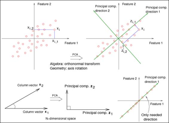
Fig. 1 A. Principal Components Analysis chooses the first PCA axis as that line that goes through the centroid, but also minimizes the square of the distance of each point to that line. Equivalently, the line goes through the maximum variation in the data. The second PCA axis also must go through the centroid and goes through the maximum variation in the data, but with a certain constraint: It must be completely uncorrelated (i.e., at right angles, or "orthogonal") to PCA axis 1. B. Consider an extreme case, (lower right), where your data all lie in one direction. Although two features represent the data, we can reduce the dimension of the dataset to one using a single linear combination of the features (as given by the first principal component). Image adapted from https://onlinecourses.science.psu.edu/stat857/node/154/ (PennState Eberly College of Science, 2019)
Clustering methods: There are two different approaches for multivariate analysis classification: the discriminant and cluster analysis. The first one is based on an a priori classification taken form canonical subjects of well-predefined classes (male/female). On the other hand, the second one approaches the intrinsic mathematical distances among the considered variables to define a conjunct of classes needed for a posteriori definition of their meaning (Kaufman & Rousseeuw, 2005; Spencer, 2013).
Cluster analysis is a technique for multivariate statistical data analysis that allows unsupervised grouping of observations into subsets (called clusters) so that observations in the same cluster are similar depending on a given criteria (Kaufman & Rousseeuw, 1990; Xu & Wunsch, 2005; Everitt, Landau, Leese, & Stahl, 2011;). “Unsupervised” implies that there is not an a priori grouped dataset to guide the grouping. Therefore, cluster analysis are suited to resolve the heterogeneity of sperm motility data in discrete subpopulations, taking special advantage of the information contained in CASA datasets (Martínez-Pastor et al., 2011).
The objective of these analysis is to assign observations to groups ("clusters") so that, within each one, the variables or attributes of interest are similar, but the groups themselves stand apart from one another based on the selected information (Everitt et al., 2011). Cluster analysis has several problems; for example, the selection of distance measure, clustering procedure, number of clusters, and the interpretation of the profile clusters and the assessment of the clustering validation.
If these analyses are applied in CASA systems, the datasets provided by CASA need to be first explored before the clustering process. Also, lack of fit of a normal distribution, skewness, outliers, extreme values, data “noise,” a weak clustering structure, and multicollinearity among different variables, have to tested first (Spencer, 2013). Nevertheless, we must take into account that datasets are expected to bear non-normal distribution and skewed variables. Thus, the presence of such features should not be automatically taken as a sign of incorrect data (Martínez-Pastor et al., 2011).
The dataset must be examined for extreme or unreliable data, which could profoundly affect clustering results (Martínez-Pastor et al., 2011). Nevertheless, it is often difficult to determine if an event is a real outlier or a real value belonging to an underrepresented cluster. Typical clustering methods of outliers - as the k-means method, which tend to group outliers in a few clusters - can be used to remove them. Moreover, some clustering methods can deal with noise or outliers as the model-based clustering (Fraley & Raftery, 2002). The CASA systems provide a high number of kinematic variables that can be redundant. That is because many of those convey similar information as the velocities (VCL, VAP, and VSL), whereas others are derived from linearity (LIN) as the VSL/VCL ratio. Therefore, it is desirable to reduce the number of variables before running the clustering algorithm, reducing both dimensionality and redundancy. Another consideration is that not all variables contribute equally in the cluster structure, and an incorrect variable selection could result in inaccurate clustering (Steinley & Brusco, 2008). A Pearson correlation analysis helps to determine subsets of highly correlated variables, suggesting redundant ones.
Clustering analysis can be a non-hierarchical or hierarchical procedure (Kaufman & Rousseeuw, 2005; Spencer, 2013). In hierarchical classifications, each sub-cluster can be formed from one larger cluster split into two, or the union of two smaller ones. In the non-hierarchical or partitional methods, the final number of clusters (k) is decided by the user before carrying out the cluster running. Then, the algorithm begins assigning the observations to the k clusters, iteratively recalculating cluster membership, and seeking for the optimal partitioning of the data. The k-means algorithm was the most used in this kind of method, but it has some drawbacks as sensitiveness to outliers and data-noise (Kaufman & Rousseeuw, 1990).
On the other hand, hierarchical clustering methods are based on a multiple-step procedure that can mainly be categorized into agglomerative (bottom-up) and divisive (top-down) procedures (Castro, Coates, & Nowak, 2004; Leonard & Droege, 2008; Wang et al., 2015) (Fig. 2). In agglomerative procedures, each subject is initially assumed to be a cluster. The two nearest clusters (based on a distance measure) are then merged at a time. This merge process continues until all the samples are clustered into one group. Consequently, a tree-like structure, known as a dendrogram, is returned. As an alternative, if the number of clusters is provided, the process of amalgamation of clusters can be terminated when the desired number is obtained. The first step of an agglomerative procedure considers all the possible mergers of two samples, which requires n (n - 1) / 2 combinations (where n depicts the number of samples) (Sharma, López, & Tsunoda, 2017). Among the agglomerative algorithms, average linkage (UPGMA) or Ward's averaging method may be more appropriate for clustering CASA systems data (Martínez-Pastor et al., 2011).
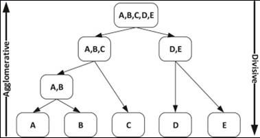
Fig. 2 Example of agglomerative and divisive hierarchical clustering. Adapted from (Everitt et al., 2011).
Divisive procedures perform clustering in the opposite way. They start by considering a group (having all samples) and divide it into two groups at each stage until all the groups comprise only a single subject (Duda, Hart, & Stork, 2001). In the first step of a divisive procedure, all the partitions of a sample set are considered, which amounts to 2n -1- 1 combinations. The number of combinations grows exponentially and practically makes divisive clustering a difficult procedure to implement. Thus, divisive procedures, which start with the entire dataset, are in general considered safer than agglomerative methods (Kaufman & Rousseeuw, 2005). Therefore, the accuracy of a divisive procedure is usually higher than that of an agglomerative procedure (Roux, 2018). However, the high computational demand (O (2n) ~ O (n 5)) of divisive procedures has severely restricted their usage (Roux, 1991). The number of bipartitions is O (n2); therefore, the complexity of one divisive step is O (n4). As the construction of the full binary hierarchy needs n - 1 steps, the overall complexity of the proposed divisive algorithms is O (n5) (Roux, 2018). This whole process involves substantial computer power. Thereby, the divisive procedure is generally not used for hierarchical clustering, remaining largely ignored in the literature (Sharma et al., 2017).
As a result, clustering analysis allows to distribute the observations (spermatozoa) in clusters (subpopulations). Sperm samples can be characterized by calculating the respective average values of the CASA parameters as the median or confidence intervals. The frequencies of each subpopulation, within males or treatments, can be estimated, obtaining different subpopulation patterns (Martínez-Pastor et al., 2011). These population frequencies can be used for further statistical analyses, such as regression, that can be used to relate subpopulations to other sperm features (Quintero-Moreno, Rigau, & Rodríguez-Gil, 2007).
Sperm subpopulation structure: It has to be remembered that the primary requirement for subpopulation analysis is that the CASA systems deliver the accurate data. The optimization of new methodological approaches, that were commented previously, suggests that the previous work developed on this topic has to be reassessed. The combination of clearly acquired image-sequences and sophisticated image processing allows to obtain reliable kinematic and morphometric sperm parameters, whose outcomes are improved datasets. This enables a better establishment of real and significant subpopulation structures within and between species (Martínez-Pastor et al., 2011).
Even with the previous technological analysis limitations, many studies have explored the use of cluster analysis to identify subpopulation patterns in sperm samples. Several works have considered kinematics data (Ortega-Ferrusola et al., 2009; Soler, García, Contell, Segervall, & Sancho, 2014; Yániz, Palacín, Vicente-Fiel, Sánchez-Nadal, & Santolaria, 2015; Yániz et al., 2018), morphometric (Aggarwal et al., 2007; Álvarez et al., 2008; Esteso et al., 2009), or a combination of both (Vásquez et al., 2016; Soler et al., 2017b).
In reference to motility, each subpopulation may be characterized accordingly to its average kinematic variables. For example, initially a subpopulation with high-velocity values and high linearity could be defined as “fast, linear”, whereas another could be defined as “slow, non-linear” (Martínez-Pastor et al., 2011). Then, the frequencies of these subpopulations can be calculated. If differences on these frequencies are detected, they can be associated to individual variations among ejaculates and individuals (Núñez-Martínez, Moran, & Peña, 2006), sperm freezability (Martínez-Pastor et al., 2005), or sperm fertility (Quintero-Moreno et al., 2003).
According to the species, different works have indicated that kinematic subpopulation structure was composed of three or four subpopulations. The presence of a “fast and linear” subpopulation has been proposed as a good indicator of sample quality, whereas a predominant “slow and non-linear” subpopulation would be a marker of poor quality (Martínez-Pastor et al., 2011). In any case, the final structure is animal dependent, and it means different animals present dissimilar subpopulation structures (Soler et al., 2017b).
Regarding morphology, the general picture is similar to motility. In human’s sperm, two (Vásquez et al., 2016) or three (Santolaria et al., 2016; Yániz et al., 2016) morphometric subpopulations were observed. In other species, a different number of subpopulations were identified; for example, three for pumas (Cucho et al., 2016) and roosters (García-Herreros, 2016), four for cats (Gutiérrez-Reinoso & García-Herreros, 2016), and five for guinea fowls (García-Herreros, 2016). Following the observed motility, each animal inside the same species showed a different subpopulation frequency, probably a consequence of its particular genetic and physiological build.
During this review, only one previous work - on foxes’ semen - was found that comprises the combination of kinematic and morphometric data for defining an integrative subpopulation structure study. Three subpopulations were observed when only kinematic or morphometric were considered, and four when combining both databases (Soler et al., 2017b). This kind of integrative work must be applied in the future, including the assessment of other parameters (DNA fragmentation, viability and membrane stability) to obtain a better comprehension of what the ejaculate is.
With this literature review, we are able to conclude that the principal goal of subpopulation structure analysis is to understand the sperm biology. Nevertheless, until now, we have just established the conceptual basis. The future must be devoted to evaluate the biological basis on the frame of sperm competition, movement along the female track, environmental effects and, finally, fertility determination.

