


 Inglês (pdf)
 Artigo em XML
 Referências do artigo
 Enviar este artigo por email
 Citado por SciELO
  Similares em
SciELO
Similares em
SciELO  uBio
uBio 
 Permalink
Revista de Biología Tropical
versão On-line ISSN 0034-7744versão impressa ISSN 0034-7744
Rev. biol. trop vol.60 supl.3 San José Nov. 2012
Global Model selection for evaluation of Climate Change projections in the Eastern Tropical Pacific Seascape
*Dirección para correspondencia:
Abstract
Two methods for selecting a subset of simulations and/or general circulation models (GCMs) from a set of 30 available simulations are compared: 1) Selecting the models based on their performance on reproducing 20th century climate, and 2) random sampling. In the first case, it was found that the performance methodology is very sensitive to the type and number of metrics used to rank the models and therefore the results are not robust to these conditions. In general, including more models in a multi-model ensemble according to their rank (of skill in reproducing 20th century climate) results in an increase in the multi-model skill up to a certain point and then the inclusion of more models degrades the skill of the multi-model ensemble. In a similar fashion when the models are introduced in the ensemble at random, there is a point where the inclusion of more models does not change significantly the skill of the multi-model ensemble. For precipitation the subset of models that produces the maximum skill in reproducing 20th century climate also showed some skill in reproducing the climate change projections of the multi-model ensemble of all simulations. For temperature, more models/simulations are needed to be included in the ensemble (at the expense of a decrease in the skill of reproducing the climate of the 20th century for the selection based on their ranks). For precipitation and temperature the use of 7 simulations out of 30 resulted in the maximum skill for both approaches to introduce the models.
Key words: Eastern Tropical Pacific Seascape, General Circulation Models, Climate Change, Precipitation, Air Surface Temperature.
Resumen
Se emplearon dos métodos para escoger un subconjunto a partir de treinta simulaciones de Modelos de Circulación General. El primer método se basó en la habilidad de cada uno de los modelos en reproducir el clima del siglo XX y el segundo en un muestreo aleatorio. Se encontró que el primero de ellos es muy sensible al tipo y métrica usada para categorizar los modelos, lo que no arrojó resultados robustos bajo estas condiciones. En general, la inclusión de más modelos en el agrupamiento de multi-modelos ordenados de acuerdo a su destreza en reproducir el clima del siglo XX, resultó en un aumento en la destreza del agrupamiento de multi-modelos hasta cierto punto, y luego la inclusión de más modelos/simulaciones degrada la destreza del agrupamiento de multi-modelos. De manera similar, en la inclusión de modelos de forma aleatoria, existe un punto en que agregar más modelos no cambia significativamente la destreza del agrupamiento de muti-modelos. Para el caso de la precipitación, el subconjunto de modelos que produce la máxima destreza en reproducir el clima del siglo XX también mostró alguna destreza en reproducir las proyecciones de cambio climático del agrupamiento de multi-modelos para todas las simulaciones. Para temperatura, más modelos/simulaciones son necesarios para ser incluidos en el agrupamiento (con la consecuente disminución en la destreza para reproducir el clima del siglo XX). Para precipitación y temperatura, el uso de 7 simulaciones de 30 posibles resultó en el punto de máxima destreza para ambos métodos de inclusión de modelos.
Palabras Clave: Corredor del Pacífico Tropical del Este, Modelos de Circulación General, Cambio Climático, Precipitación, Temperatura superficial del aire.
The impacts of anthropogenic forcings in the Earth’s climate are a reality that is already affecting and will continue to affect human and environmental systems (Barnett et al. 2008, Pierce et al. 2008, Hidalgo et al. 2009). Because anthropogenic causes and consequences represented by modifications of the natural climate patterns are lagged by a number of years (or even decades), it is necessary to assess the state of future climates with some lead time using numerical global climate models, also known as General Circulation Models (GCMs). The final objective is that the GCMs would be used to estimate a range of possible climate change projections, given the uncertainties in the future climate forcing data and the limitations of the models in simulating climate in a realistic manner. This exercise is therefore crucial for guiding mitigation and adaptation actions associated with significant changes in policy and/or infrastructure which require some time for implementation (Amador & Alfaro 2009).
Unfortunately, the GCM climate raw data alone are not generally useful for regional impact studies (Hidalgo et al. 2009, Maurer & Hidalgo 2008, Pierce et al. 2009). Not only does the current generation of models provide a much coarser spatial (and sometimes temporal) resolution that in many cases is needed, but also climate data have to be interpreted in terms of the impacts in diverse sectors (i.e. water supply, agriculture, hydropower generation, wildfire potential, social and economic aspects, public health) using statistical or physical models for downscaling the GCM climate data to a finer resolution and/or including additional analysis or models for the estimation of these impacts (Amador & Alfaro 2009). For reasons of simplicity or for limitations in processing capacity or resources, this process of transforming the GCM climate data into regional climate change impacts assessments have been usually done using a subset of a few models from the range of all available models in the repositories of GCM data (i.e. Cayan et al. 2008). Therefore, selecting the models to use for a certain region needs to be evaluated using logical criteria (see examples in Pierce et al. 2009, Cayan et al. 2008, Brekke et al. 2008). This article presents a comparison between two methods of selecting models. The first method consists of selecting the models based on their performance of reproducing 20th century’s climate, and the second method is simply choosing the models at random. In particular, the main objective of the article is to determine how many simulations are needed to be selected to form an n-ensemble from a total of N=30 simulations in order to optimize the skill in reproducing statistics of the climate of the 20th century or to obtain similar climate change projections of temperature and precipitation changes as the multi-model ensemble of the N models (MMEN) at two projection horizons: 2000-2049 and 2050-2099.
Previous studies have suggested that risk assessment could be influenced by the accounting for model credibility, and that this assessment is also sensitive to projected quantity (Brekke et al. 2008). Like Brekke et al. (2008) we are interested in determining if selecting fewer simulations than the total available in the dataset results in different climate change projections compared to the ensemble of all available simulations (in our case MMEN), but our approach is somewhat different than Brekke’s. We are interested in determining if the work spent of calculating the weights of the simulations for culling is worth it, or if instead a random selection of models results in a similar subset of n=nr models. (Also we are interested in determining if nr << N or not). Pierce et al. (2009) already showed that model selection using performance metrics showed no systematically different conclusions than random sampling on detection and attribution (D&A) analysis of January-February-March (JFM) temperature for the western United States (US) data. The authors also demonstrated that multi-model ensembles showed superior results compared to individual models and that enough realizations should be chosen to account for natural climate variability in D&A studies. The authors found that model skill tend to asymptote after a few numbers of models are considered in the ensemble, but their work does not refer to 21st century climate projections. They mention, however, that the ordering the models by performance has the effect of ordering them by climate sensitivity (during the 20th century) more than would be expected by chance, with the better models having higher sensitivities.
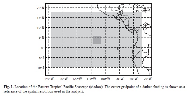
The area of study of this article is the Eastern Tropical Pacific Seascape (ETPS; Fig. 1). It is a very important region covering more than 2 million km2, the national waters of many countries, immense concentration of endangered pelagic species, unique variety of tropical and temperate marine life, and four UNESCO World Heritage Sites, including Costa Rica’s Isla del Coco National Park (Cortés 2008; Henderson et al. 2008). The ETPS is also an important center of action of El Niño-Southern Oscillation (ENSO) phenomena (Alfaro 2008; Quirós-Badilla & Alfaro 2009).
In the next section the used data will be described, then the analysis is divided in three parts: 1) Part I is the selection based on performance criteria of the models on reproducing the 20th century climate features, 2) Part II is the selection at random, and 3) Part III is the analysis of the results in terms of the 21st century projections. The discussion of the results will be presented in the last section.
Data
Global climate simulations corresponding to monthly precipitation and temperature runs for the climate of the 20th century (known as 20c3m runs) and climate projections for the 21st century for the A1B greenhouse gas emission scenario were obtained from the US Lawrence Livermore National Laboratory Program for Climate Model Diagnosis and Intercomparison (PCMDI 2010) and from the Intergovernmental Panel on Climate Change (IPCC 2010). These data were collected as a response of an activity of the World Climate Research Programme (WCRP) of the World Meteorological Organization (WMO) and constitutes phase 3 of the Coupled Model Intercomparison Project (CMIP Phase 3) in support of research relied on by the 4th Assessment Report (AR4) of the IPCC (Meehl et al. 2007). Redundant runs from the PCMDI and IPCC datasets were compared and discarded. Only those models that had complete runs for all of the following periods were considered in the analysis: a) climate of the 20th century or 20c3m type of simulations (covering the time period 1950 to 1999), b) the climate change projection for the horizon 1 or CC1 (2000 to 2049), and c) the climate change projection for the horizon 2 or CC2 (2050 to 2099). Some of the models that had more than one climate change realization were also considered in the analysis. There were a total of N=30 simulations that met these requirements. The list of models and runs can be found in Table 1.
Global climate change data from their original resolution were interpolated to the resolution of the coarsest model (2o latitude x 5o longitude) by the nearest grid-point method, but considering separate interpolations for the ocean and land grid-points according to the individual land-sea masks of the models. The data were visually inspected at selected grid- points. The data were also changed to the same units and same file format for the rest of the analysis.
Performance of the GCM 20c3m precipitation and temperature data was estimated in reference to the US National Center of Environmental Prediction (NCEP) and US National Center for Atmospheric Research (NCAR) Reanalysis (Kalnay et al. 1996), hereinafter the Reanalysis. The data for comparison covers the period from 1950 to 1999. It should be mentioned that the precipitation of the Reanalysis is modeled (not observed) and thus it may have larger errors than the temperature data.
Part I
Selection of models using performance metrics
In this part, the GCMs were culled according to their performance on reproducing 20th century climate, as represented in the Reanalysis.
Metrics
Several metrics were used to determine the performance of the models on reproducing 20th century statistics for the first part of the analysis (selection of models using performance metrics). The metrics were divided in three categories: 1) metrics on the mean, 2) metrics on the variability and 3) metrics on the spectral characteristics. There are 13 metrics of the mean type corresponding to the mean of the annual averages (denoted by mY) plus the means for each of the 12 individual months (climatologies) of climate patterns (denoted by mJ, mF, … mD) over the shaded region (Fig. 1). In a similar fashion there are 13 metrics on the variability corresponding to the standard deviations of the 13 annual and monthly averages defined before (denoted by sY, sJ, ...sD) . Finally, there are two spectral types of metrics: the first was calculated by running a 2 to 8 year elliptical band-pass filter (Ginde & Noronha 2012) on the annual precipitation or temperature time-series at each grid-point and calculating the ratio of the standard deviation of the filtered data to the standard deviation of the unfiltered data. This metric is a measure of how much “high-frequency” climate variability (a large part related to ENSO) is captured by the model (denoted as fH). The second spectral metric is defined similarly, except that it captures the “low frequency” climate variability contained in the spectral band between 9 and 20 years (denoted as fL). There are no global climate metrics such as ENSO, Pacific Decadal Oscillation, Atlantic Multidecadal Oscillation or corresponding tele-connection metrics in the present analysis as in Brekke et al. (2008). Because the study region is almost at the equatorial Pacific, it was considered here that a large part of the dominating ENSO signal is represented in the temperature and precipitation metrics already (Alfaro 2008; Quirós-Badilla & Alfaro 2009) and that a similar analysis of the determination of nr due to global tele-connections will follow in a separate article.
Skill Score
Following Pierce et al. (2009), the degree of similarity between any two climate patterns (for example between the Reanalysis metric and the same metric from one of the GCM simulations) was calculated using the Skill Score (SS) defined by:
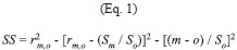
where rm,o is the Pearson´s spatial correlation between modeled (i.e. GCM) and “observed” (i.e. Reanalysis) patterns, sm and so are the sample spatial standard deviations for the modeled and observed patterns respectively. The ratio sm/so is denoted as g in following sections. The m and o over-bars correspond to the spatial average of the modeled and observed climate patterns respectively. SS varies from minus infinity (no skill) to 1 (perfect match between the patterns). Zero SS values correspond to cases in which the mean of the observations is reproduced correctly by the model in a certain region, but only as a featureless uniform pattern (Pierce et al. 2009). Inspection of the right hand side of Equation 1 shows that SS is composed of three squared terms, and therefore SS can also be expressed as:
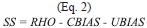
where RHO is the square of the spatial correlation between the observed and modeled patterns; and CBIAS and UBIAS are the Conditional and Unconditional Biases respectively (see Pierce et al. 2009). Note that SS not only reflects correlation coherence between the pat- terns but also biases play an important role in SS’s calculation.
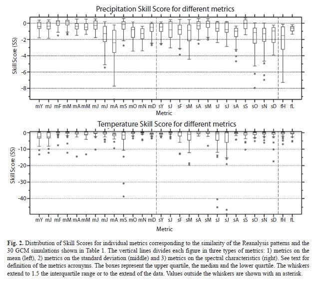
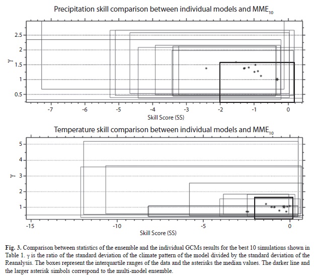
The spreads of the SS values calculated for individual models and by individual metrics are shown in Figure 2. As can be seen precipitation SSs are generally lower than for temperature. This suggests that precipitation is not reproduced well in this region of the world by many of the GCMs, compared to the Reanalysis. Temperature mean type of metrics showed good skill for many models, even for the spectral type of metrics. This calculation of metrics for each individual model is necessary in order to rank the models. The rank is actually computed by combining the SSs of individual metrics through calculation of the Euclidean distances (hereafter denoted by ΔSS) between the obtained SSs for each metric and the “perfect” or “optimal” vector SS=(1,1,1,…1). In order to determine the sensitivity to the type of metrics used, three types of Euclidean distances were calculated: 1) only the precipitation metrics were used in the calculation of SS, 2) the precipitation and temperature metrics were used and 3) only the temperature metrics were used. These distances were used to rank the models and for determining the order on which the models form the ensemble in groups of n=1,2,...30. That is, with the exception of Figures 2 and 3 the average SSs and SSs will always be computed for model ensembles. The reason for this is that, as mentioned in Pierce et al. (2009), the model ensembles are generally better than the individual model results; a result also partially suggested in Figure 3. For precipitation the median SS for the simple model ensemble at using the best 10 models n=10 (MME10) is always better than the results for the best 10 individual models (Fig. 3); and also the MME10 showed g values close to the unity. Models or ensembles with g closer to the unity have a desirable feature that is discussed in Pierce et al. 2009. For temperature, some of the individual models showed better median SS.
Selection of model ensembles
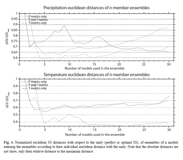
Each model and metric has a particular SS. In order to determine the performance of any single particular model at representing all of the metrics, the Euclidean distance or ΔSS between the SSs of all the metrics of that model and the “perfect” or “optimal” vector SS=(1,1,1,...1) of length nm, where nm=number of metrics used, was computed. These distances were used to rank the models according to their distance to form multi-model n-ensembles (MMEn) composed of the best n individual models introduced in increasing ranking of ΔSS. The normalized Euclidean distances or ΔSS/ΔSSmax for each resulting ensemble are shown in Figure 4, using different variables in the calculation of the metrics. In Figure 4 ΔSSmax is the ΔSS that showed the maximum deviation from the optimum vector SS=(1,1,1,…1). As mentioned previously, regardless of the variable to be analyzed, the calculation of the Euclidean distances was performed using precipitation metrics only (nm=13+13+2=28, corresponding to the mean, variability and spectral types of metrics mentioned before), precipitation and temperature metrics (nm=28*2=56) and temperature metrics only (nm=28). Note that in Figure 4, only the normalized distances are of interest, and the different curves are not directly comparable to each other. From Figure 4 and for precipitation and temperature metrics (solid curves), it can be seen that the inclusion of more models generally increases the skill of the n-ensemble to reproduce the Reanalysis precipitation and temperature patterns up to a certain number of models and then the skill generally decreases when the worse models are included in the ensembles. Therefore, there is an optimum number of models to be included in the ensembles in order to obtain the greatest skill. Note also that there is a strong dependence of the results on the type of metrics used and whether precipitation, temperature or both type of patterns are used to determine the order in which the models are introduced in the ensembles. Thus, it is clear that the variables included in the calculation of the metrics significantly influences the results. In fact, the type of metrics used also influenced the results, as the analysis was repeated using all possible combinations of type of metrics (mean, variability and spectral) which resulted in different results (not shown). This problem was also mentioned in Pierce et al. (2009) and Brekke et al. (2008). Precipitation’s ΔSS/ΔSSmax is the lowest (for the precipitation and temperature metrics) at around n=nr=7 (the lowest point for the solid curve of top Figure 4), and temperature results show a lowest distance value at n=nr=7 (the lowest point for the solid curve of bottom Figure 4).
Part II
Random selection of models
In this part of the analysis, the models form ensembles of size n, chosen randomly.
Selecting a representative sample
In order to obtain statistical significance in the results it is necessary to obtain a certain sample from a population of possible combinations of N models, taken in ensembles of n members. The possible number of combinations for ensembles of n simulations from a total of N=30 individual possible simulations is given in any elementary combinatorics text-book by (see for example Spiegel 1998):
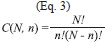
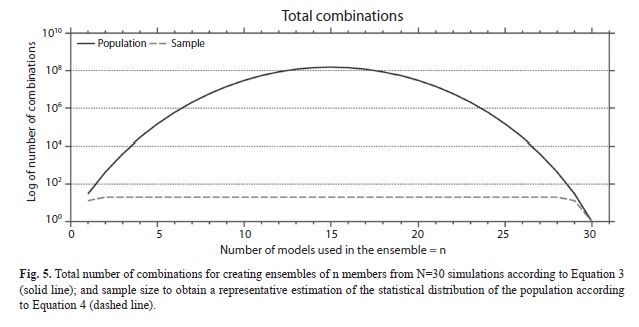
C(N,n) increases very rapidly until the maximum at n=15 where it reaches values higher than 1x10⁸ possible combinations and then decreases rapidly to become equal to 1 for n=N=30 (Fig. 5). Since the calculation of all possible combinations is extremely large, representative samples of the population of size SC(N,n) were taken that resulted in the same statistical distribution as the population with a 95% confidence level using the following formulas from Israel (2009):

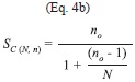
where “ceil” is the rounding to the higher integer, Z2 is the abscissa of the normal curve that cuts off an area at the tails (1-confidence level, e.g. 95%), p is equal to the estimate proportion that is present in the population, while the value of q is given by q=1-p. Since p has an unknown aspect, the most conservative option for p and q (p=q=0.5) was used as it produces the largest no value. Also e=0.05 is the error that is anticipated to be committed. Inspection of the equation showed that it converges to a plateau very rapidly (Fig. 5).
Equation 4 was tested using a Monte Carlo simulation for ensembles of sizes n=1 to n=6. The SS distributions for the populations were computed, and 100 000 samples of SC(N,n) combinations of n simulations were computed. The samples and the population distributions were compared using a Kolmogorov–Smirnov or K–S test. It was verified that the error committed was below 5% and therefore this serves as an indication that Equation 4 gives useful estimations of the needed sample size.
Selection of model ensembles
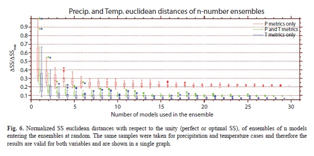
In Figure 6 the results for the random selection of simulations are shown. The same samples were selected for precipitation and temperature and therefore the results for both variables are the same in Figure 6. At around n=nr=7 there is a plateau in the values of ΔSS/ΔSSmax, suggesting that the inclusion of more models at random does not substantially improve the skill beyond that point.
Part III
Implication for climate change projections
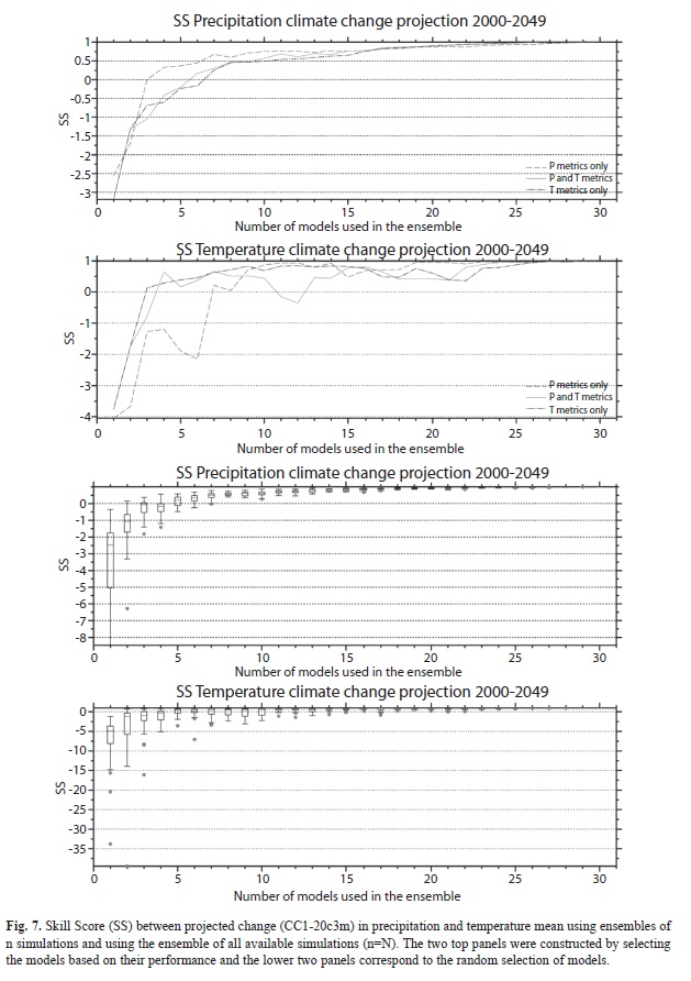
In this section we are interested in determining whether the nr values obtained previously in Parts I and II result in similar projected precipitation and temperature change for two climate change horizons: CC1 (2000 to 2049) and CC2 (2050 to 2099). The difference in the mean January to December future conditions (CC1 or CC2) and the 20c3m “historical” scenarios were computed for the same ensembles determined in Figure 4 and Figure 6 (See Brekke et al. 2008 for a discussion on how the climate change variable to be used affects the results). The SSs between the climate change patterns of each individual n-member ensemble and the MMEN for the two climate change horizons are shown in Figures 7 and 8. For the CC1 climate change horizon (and for the precipitation and temperature metrics), precipitation ensembles using the selection based on performance is positive (and stays positive) at around n=ncc1=6. In other words, the ensemble of 6 models (or more) is needed in order to guarantee that there is some skill in reproducing the climate change pattern of the MMEN. This also implies that the most conservative number of models used to create the ensemble between nr=7 and ncc1=6 would ensure that 1) the best performance of the model in reproducing the features of the “historical” period as shown in the Reanalysis is found and 2) the ensemble also has some skill in reproducing the same climate projection using as basis the ensemble of all available simulations. As can be seen both numbers of models are very similar and with n=7 the maximum skill in reproducing 20th century climate is found, along with some skill in reproducing the climate change patterns of the MMEN. In the case of precipitation random sampling, all the simulations have SSs greater than zero at n=ncc1=8, while the less conservative value of nr=7 found in Part II suggests that the constraint of having some skill in reproducing the climate change of the MMEN is more conservative. Note that the normalized Euclidean distances shown on figures 4 and 6, do not say anything about the absolute distances and therefore both figures are not comparable to each other. But in Figures 7 and 8, the use of the Skill Score (Equation 1) to test the similarity between the projected climate of the MMEn and MMEN allow comparison between the charts for any single climatic parameter (precipitation or temperature) and climate change scenario.
In the case of temperature, the creation of ensembles using the performance criteria suggests that n=ncc1=13 is needed (point where solid line is positive and stays positive in second panel from the top in Figure 7) in order to obtain positive SS values, contrasting with the n=nr=7 found in Part I of the analysis. This suggests that if the sampling is based on performance criteria, the ensemble of the best 13 models are needed in order to guarantee some skill in reproducing the climate change patterns of the multi-model ensemble, and that the maximum skill is achieved. In the case of random sampling, n=ncc1=15 is needed, in contrast with n=nr=6 found before. In Table 2 a summary of the results is presented for both climate change horizons. The results are very similar and support the same conclusions discussed in this part of the analysis.
Discussion
When selecting a subset of simulations and/or models for a regional study, it is very common to use some performance criteria to determine which simulations to use. Consistent with other studies, it was found here, that the selection and the results are very sensitive to the metrics used to rank the simulations. In this study, this multi-model ensemble of all available simulations was used as a benchmark to compare the results of the climate change simulations with the objective of determining if using a smaller subset of simulations results in very different climate projections.
The results showed that culling the models based on performance criteria or on random sampling, results in future precipitation projections that have some similarity to the projections obtained from the MMEN. For temperature, more models are needed to be added to the ensemble to guarantee skill in reproducing climate change patterns of the MMEN. It could be argued that the use of the MMEN as a benchmark is not justified as it contains models with very low skill in reproducing observations, but it is assumed here that as more simulations are included in the ensemble, the more noise is going to be filtered out and therefore this benchmark has superior characteristic than the multi-model ensemble of a subset of n<N simulations or MMEn.
Among other aspects discussed here, this assumption depends also on the sensitivity of the models in the area of study and the parameter used. This particular area showed low sensitivity (in particular to precipitation) when the skill of individual models were computed (Fig. 2). Moreover the region also shows no clear and consistent trend in precipitation means during the projected 21st century climate (Maldonado & Alfaro 2011, Hidalgo & Alfaro 2012), although it does show an evident warming tendency (Hidalgo & Alfaro 2012). Studies in other regions may provide more information regarding the size of the ensembles needed in other cases.
Conclusion
The inclusion of models in the multi-model ensemble based on their rank of reproducing 20th century climate showed great variability depending on which type of metrics were used to determine their rank. For the precipitation variable, ranks based on precipitation and temperature metrics (solid curve of top panel of Figure 4) showed that inclusion of models reach a maximum skill (lowest ΔSS/ΔSSmax) at around 7 models. When the models are introduced at random we found that around that same number of models the maximum skill is found. Therefore it seems that the inclusion of around 7 models out of 30 is the optimum number of models to produce an ensemble if the ranks are based on precipitation and temperature metrics. Note that it is not suggested that the 7 models culled according to their rank or selected at random have the same absolute skill; it only means that beyond 7 models there is not much change in the skill (or actually there is a degradation of the skill caused by models that do not contribute to improve the overall skill of the MMEn). If we use temperature metrics to determine the rank of the models for the precipitation variable (dark dash dotted line of top Figure 4), the maximum skill is found at the MMEN. It is difficult to interpret what this means in terms of the distribution of the skill of the MMEn. For the temperature variable, if we use precipitation and temperature metrics (solid curves of bottom Figure 4), when we reach 7 models there is a point of maximum skill (lowest ΔSS/ΔSSmax) and then the skill changes slightly until the 30 models are introduced in the MMEN. This is the same than the 7 randomly selected models that can be combined to reach the plateau in skill in Figure 6. When the precipitation patterns are used to determine the ranks of the models to be used to compute the skill for the temperature variable, the maximum skill is reach at around 21 models (light dashed line of bottom Figure 4). It can be concluded from all this that in general there is an optimum number of models/ simulations to be used in the ensemble and that number could be significantly lower than the total number of models/simulations. However, finding this optimum number is difficult as it is heavily dependent on how the models are introduced into the multi-model ensemble and on the type of metrics used. This however, does not guarantee that the climate change patterns produced by the MMEn are similar to the patterns produced by the MMEN as this has to be determined in a separate analysis.
Acknowledgments
This work was partially financed by projects (808-A9-180, 805-A9-224, 805-A9-532, 808-B0-092, 805-A9-742, 805-A8-606 and 808-A9-070) from the Center for Geophysical Research (CIGEFI) and the Marine Science and Limnology Research Center (CIMAR) of the University of Costa Rica (UCR). Thanks for the logistics support of the School of Physics of UCR. The authors were also funded through an Award from Florida Ice and Farm Company (Amador, Alfaro and Hidalgo). HH is also funded through a grant from the Panamerican Institute of Geography and History (GEOF.02.2011). The authors are obliged to André Stahl from UCR who processed much of the raw GCM data and Mary Tyree from Scripps Institution of Oceanography who provided the land-sea masks of the models. Also to María Fernanda Padilla and Natalie Mora for their help with the data base. Finally, to the National Council of Public University Presidents (CONARE), for the support of a FEES project “Interacciones oceáno-atmósfera y la biodiversidad marina del Parque Nacional Isla del Coco” (project 808-B0-654, UCR). We would like to thank two anonymous reviewers and Dr. Javier Soley that helped improve the quality of this article.
References
Alfaro, E. 2008. Ciclo diario y anual de variables troposféricas y oceánicas en la Isla del Coco, Costa Rica. Rev. Biol. Trop. 56 (Supl. 2): 19-29. [ Links ]
Amador, J.A. & E.J. Alfaro. 2009. Métodos de reducción de escala: Aplicaciones al tiempo, clima, variabilidad climática y cambio climático. Rev. Iberoamer. Econ. Ecol. 11: 39-52. [ Links ]
Barnett, T., D.W. Pierce, H. Hidalgo, C. Bonfils, B.D. Santer, T. Das, G. Bala, A.W. Wood, T. Nazawa, A. Mirin, D. Cayan, & M. Dettinger, 2008, Human-induced changes in the hydrology of the western United States. Science 319: 1080-1083. [ Links ]
Brekke, L.D., M.D. Dettinger, E.P. Maurer & M. Anderson. 2008. Significance of model credibility in estimating climate projection distributions for regional hydro- climatological risk assessments. Clim. Change 89: 371-394. [ Links ]
Cayan, D.R., E.P. Maurer, M.D. Dettinger, M. Tyree & K. Hayhoe. 2008. Climate change scenarios for the California region. Clim. Change 87: S21-S42. [ Links ]
Cortés, J. 2008. Historia de la investigación marina de la Isla del Coco, Costa Rica. Rev. Biol. Trop. 56 (Supl. 2): 1-18. [ Links ]
Guinde S. V. & J.A.N. Noronha. 2012, Design of IRR filters (last visit: July 4th, 2012, available at http://www.ee.vt.edu/~jnoronha/dsp_proj2_report.pdf). [ Links ]
Henderson, S., A.M. Rodríguez & R. McManus. 2008. A new future for marine conservation. Eastern Tropical Pacific Seascape. Technical Document: 4 p. (last visit: May 6th, 2010, available at http://www.conservation.org/). [ Links ]
Hidalgo, H.G., & E.J. Alfaro. 2012. Some physical and socio-economic aspects of climate change in Central America. Prog. Phys. Geog. 36: 379-399. [ Links ]
Hidalgo, H.G., T. Das, M.D. Dettinger, D.R. Cayan, D.W. Pierce, T.P. Barnett, G. Bala, A. Mirin, A.W. Wood, C. Bonfils, B.D. Santer & T. Nozawa. 2009. Detection and attribution of streamflow timing changes to Climate Change in the Western United States. J. Clim. 22: 3838-3855. [ Links ]
IPCC. 2010. The Intergovernmental Panel on Climate Change. The IPCC Data Distribution Centre. Available at http://www.ipcc-data.org/. Accessed January to July 2010. [ Links ]
Israel G.D. 2009. Determining Sample Size. University of Florida Institute of Food and Agricultural Sciences (IFAS) Extension publication. PEOD6. 7 pp. [ Links ]
Kalnay, E., M. Kanamitsu, R. Kistler, W. Collins, D. Deaven, L. Gandin, M. Iredell, S. Saha, G. White, J. Woollen, Y. Zhu, A. Leetmaa & R. Reynolds. 1996. The NCEP/NCAR 40-Year Reanalysis Project. Bull. Amer. Meteor. Soc. 77: 437-471. [ Links ]
Maldonado, T. & E. Alfaro. 2011. Revisión y comparación de escenarios de cambio climático para el Parque Nacional Isla del Coco, Costa Rica. Rev. Biol. Trop. This volume. [ Links ]
Maurer, E.P. & H.G. Hidalgo. 2008. Utility of daily vs. monthly large-scale climate data: an intercomparison of two statistical downscaling methods. Hydrol. Earth Syst. Sci. 12: 551-563. [ Links ]
Meehl G.A., C. Covey, T. Delworth, M. Latif, B. McAvaney, J. F. B. Mitchel, R.J. Stouffer & K.E. Taylor. 2007. The WRCP CMIP3 multimodel dataset. Bulletin of the American Meteorological Society. DOI:10.1175/BAMS-88-9-1383: 1383-1394. [ Links ]
PCMDI. 2010. Lawrence Livermore National Laboratory Program for Climate Model Diagnosis and Intercomparison. Available at http://www-pcmdi.llnl.gov/. Accessed August 2009 to July 2010. [ Links ]
Pierce D.W., T.P. Barnett, H.G. Hidalgo. T. Das, C. Bonfils, B. Sander, G. Bala, M. Dettinger, D. Cayan & A. Mirin. 2008. Attribution of declining western US snowpack to human effects. J. Clim, 21: 6425-6444. [ Links ]
Pierce, D.W., T.P. Barnett, B.D. Santer & P.J. Gleckler. 2009. Selecting global climate models for regional climate change studies. Proc. Nat. Acad. Sci. USA 106: 8441-8446. [ Links ]
Quirós-Badilla, E. & E. Alfaro. 2009. Algunos aspectos relacionados con la variabilidad climática en la Isla del Coco, Costa Rica. Rev. Clim. 9: 33-34. [ Links ]
Spiegel, M. 1998. Estadística. Serie Shaum. 2da ed. McGraw-Hill, México D.F., México. 556 p. [ Links ]
*Corespondencia: Hugo G. Hidalgo: Escuela de Física, Universidad de Costa Rica, 11501-2060 San José, Costa Rica; hugo.hidalgo@ucr.ac.cr. Centro de Investigaciones Geofísicas, Universidad de Costa Rica, 11501-2060 San José, Costa Rica.
Eric J. Alfaro: Escuela de Física, Universidad de Costa Rica, 11501-2060 San José, Costa Rica; erick.alfaro@ucr.ac.cr. Centro de Investigaciones Geofísicas, Universidad de Costa Rica, 11501-2060 San José, Costa Rica. Centro de Investigación en Ciencias del Mar y Limnología, Universidad de Costa Rica, 11501-2060, San José, Costa Rica.
1. Escuela de Física, Universidad de Costa Rica, 11501-2060 San José, Costa Rica; hugo.hidalgo@ucr.ac.cr, erick.alfaro@ucr.ac.cr..
2. Centro de Investigaciones Geofísicas, Universidad de Costa Rica, 11501-2060 San José, Costa Rica.
3. Centro de Investigación en Ciencias del Mar y Limnología, Universidad de Costa Rica, 11501-2060, San José, Costa Rica.
*Dirección para correspondencia:
Abstract
Two methods for selecting a subset of simulations and/or general circulation models (GCMs) from a set of 30 available simulations are compared: 1) Selecting the models based on their performance on reproducing 20th century climate, and 2) random sampling. In the first case, it was found that the performance methodology is very sensitive to the type and number of metrics used to rank the models and therefore the results are not robust to these conditions. In general, including more models in a multi-model ensemble according to their rank (of skill in reproducing 20th century climate) results in an increase in the multi-model skill up to a certain point and then the inclusion of more models degrades the skill of the multi-model ensemble. In a similar fashion when the models are introduced in the ensemble at random, there is a point where the inclusion of more models does not change significantly the skill of the multi-model ensemble. For precipitation the subset of models that produces the maximum skill in reproducing 20th century climate also showed some skill in reproducing the climate change projections of the multi-model ensemble of all simulations. For temperature, more models/simulations are needed to be included in the ensemble (at the expense of a decrease in the skill of reproducing the climate of the 20th century for the selection based on their ranks). For precipitation and temperature the use of 7 simulations out of 30 resulted in the maximum skill for both approaches to introduce the models.
Key words: Eastern Tropical Pacific Seascape, General Circulation Models, Climate Change, Precipitation, Air Surface Temperature.
Resumen
Se emplearon dos métodos para escoger un subconjunto a partir de treinta simulaciones de Modelos de Circulación General. El primer método se basó en la habilidad de cada uno de los modelos en reproducir el clima del siglo XX y el segundo en un muestreo aleatorio. Se encontró que el primero de ellos es muy sensible al tipo y métrica usada para categorizar los modelos, lo que no arrojó resultados robustos bajo estas condiciones. En general, la inclusión de más modelos en el agrupamiento de multi-modelos ordenados de acuerdo a su destreza en reproducir el clima del siglo XX, resultó en un aumento en la destreza del agrupamiento de multi-modelos hasta cierto punto, y luego la inclusión de más modelos/simulaciones degrada la destreza del agrupamiento de multi-modelos. De manera similar, en la inclusión de modelos de forma aleatoria, existe un punto en que agregar más modelos no cambia significativamente la destreza del agrupamiento de muti-modelos. Para el caso de la precipitación, el subconjunto de modelos que produce la máxima destreza en reproducir el clima del siglo XX también mostró alguna destreza en reproducir las proyecciones de cambio climático del agrupamiento de multi-modelos para todas las simulaciones. Para temperatura, más modelos/simulaciones son necesarios para ser incluidos en el agrupamiento (con la consecuente disminución en la destreza para reproducir el clima del siglo XX). Para precipitación y temperatura, el uso de 7 simulaciones de 30 posibles resultó en el punto de máxima destreza para ambos métodos de inclusión de modelos.
Palabras Clave: Corredor del Pacífico Tropical del Este, Modelos de Circulación General, Cambio Climático, Precipitación, Temperatura superficial del aire.
The impacts of anthropogenic forcings in the Earth’s climate are a reality that is already affecting and will continue to affect human and environmental systems (Barnett et al. 2008, Pierce et al. 2008, Hidalgo et al. 2009). Because anthropogenic causes and consequences represented by modifications of the natural climate patterns are lagged by a number of years (or even decades), it is necessary to assess the state of future climates with some lead time using numerical global climate models, also known as General Circulation Models (GCMs). The final objective is that the GCMs would be used to estimate a range of possible climate change projections, given the uncertainties in the future climate forcing data and the limitations of the models in simulating climate in a realistic manner. This exercise is therefore crucial for guiding mitigation and adaptation actions associated with significant changes in policy and/or infrastructure which require some time for implementation (Amador & Alfaro 2009).
Unfortunately, the GCM climate raw data alone are not generally useful for regional impact studies (Hidalgo et al. 2009, Maurer & Hidalgo 2008, Pierce et al. 2009). Not only does the current generation of models provide a much coarser spatial (and sometimes temporal) resolution that in many cases is needed, but also climate data have to be interpreted in terms of the impacts in diverse sectors (i.e. water supply, agriculture, hydropower generation, wildfire potential, social and economic aspects, public health) using statistical or physical models for downscaling the GCM climate data to a finer resolution and/or including additional analysis or models for the estimation of these impacts (Amador & Alfaro 2009). For reasons of simplicity or for limitations in processing capacity or resources, this process of transforming the GCM climate data into regional climate change impacts assessments have been usually done using a subset of a few models from the range of all available models in the repositories of GCM data (i.e. Cayan et al. 2008). Therefore, selecting the models to use for a certain region needs to be evaluated using logical criteria (see examples in Pierce et al. 2009, Cayan et al. 2008, Brekke et al. 2008). This article presents a comparison between two methods of selecting models. The first method consists of selecting the models based on their performance of reproducing 20th century’s climate, and the second method is simply choosing the models at random. In particular, the main objective of the article is to determine how many simulations are needed to be selected to form an n-ensemble from a total of N=30 simulations in order to optimize the skill in reproducing statistics of the climate of the 20th century or to obtain similar climate change projections of temperature and precipitation changes as the multi-model ensemble of the N models (MMEN) at two projection horizons: 2000-2049 and 2050-2099.
Previous studies have suggested that risk assessment could be influenced by the accounting for model credibility, and that this assessment is also sensitive to projected quantity (Brekke et al. 2008). Like Brekke et al. (2008) we are interested in determining if selecting fewer simulations than the total available in the dataset results in different climate change projections compared to the ensemble of all available simulations (in our case MMEN), but our approach is somewhat different than Brekke’s. We are interested in determining if the work spent of calculating the weights of the simulations for culling is worth it, or if instead a random selection of models results in a similar subset of n=nr models. (Also we are interested in determining if nr << N or not). Pierce et al. (2009) already showed that model selection using performance metrics showed no systematically different conclusions than random sampling on detection and attribution (D&A) analysis of January-February-March (JFM) temperature for the western United States (US) data. The authors also demonstrated that multi-model ensembles showed superior results compared to individual models and that enough realizations should be chosen to account for natural climate variability in D&A studies. The authors found that model skill tend to asymptote after a few numbers of models are considered in the ensemble, but their work does not refer to 21st century climate projections. They mention, however, that the ordering the models by performance has the effect of ordering them by climate sensitivity (during the 20th century) more than would be expected by chance, with the better models having higher sensitivities.
The area of study of this article is the Eastern Tropical Pacific Seascape (ETPS; Fig. 1). It is a very important region covering more than 2 million km2, the national waters of many countries, immense concentration of endangered pelagic species, unique variety of tropical and temperate marine life, and four UNESCO World Heritage Sites, including Costa Rica’s Isla del Coco National Park (Cortés 2008; Henderson et al. 2008). The ETPS is also an important center of action of El Niño-Southern Oscillation (ENSO) phenomena (Alfaro 2008; Quirós-Badilla & Alfaro 2009).
In the next section the used data will be described, then the analysis is divided in three parts: 1) Part I is the selection based on performance criteria of the models on reproducing the 20th century climate features, 2) Part II is the selection at random, and 3) Part III is the analysis of the results in terms of the 21st century projections. The discussion of the results will be presented in the last section.
Data
Global climate simulations corresponding to monthly precipitation and temperature runs for the climate of the 20th century (known as 20c3m runs) and climate projections for the 21st century for the A1B greenhouse gas emission scenario were obtained from the US Lawrence Livermore National Laboratory Program for Climate Model Diagnosis and Intercomparison (PCMDI 2010) and from the Intergovernmental Panel on Climate Change (IPCC 2010). These data were collected as a response of an activity of the World Climate Research Programme (WCRP) of the World Meteorological Organization (WMO) and constitutes phase 3 of the Coupled Model Intercomparison Project (CMIP Phase 3) in support of research relied on by the 4th Assessment Report (AR4) of the IPCC (Meehl et al. 2007). Redundant runs from the PCMDI and IPCC datasets were compared and discarded. Only those models that had complete runs for all of the following periods were considered in the analysis: a) climate of the 20th century or 20c3m type of simulations (covering the time period 1950 to 1999), b) the climate change projection for the horizon 1 or CC1 (2000 to 2049), and c) the climate change projection for the horizon 2 or CC2 (2050 to 2099). Some of the models that had more than one climate change realization were also considered in the analysis. There were a total of N=30 simulations that met these requirements. The list of models and runs can be found in Table 1.
Global climate change data from their original resolution were interpolated to the resolution of the coarsest model (2o latitude x 5o longitude) by the nearest grid-point method, but considering separate interpolations for the ocean and land grid-points according to the individual land-sea masks of the models. The data were visually inspected at selected grid- points. The data were also changed to the same units and same file format for the rest of the analysis.
Performance of the GCM 20c3m precipitation and temperature data was estimated in reference to the US National Center of Environmental Prediction (NCEP) and US National Center for Atmospheric Research (NCAR) Reanalysis (Kalnay et al. 1996), hereinafter the Reanalysis. The data for comparison covers the period from 1950 to 1999. It should be mentioned that the precipitation of the Reanalysis is modeled (not observed) and thus it may have larger errors than the temperature data.
Part I
Selection of models using performance metrics
In this part, the GCMs were culled according to their performance on reproducing 20th century climate, as represented in the Reanalysis.
Metrics
Several metrics were used to determine the performance of the models on reproducing 20th century statistics for the first part of the analysis (selection of models using performance metrics). The metrics were divided in three categories: 1) metrics on the mean, 2) metrics on the variability and 3) metrics on the spectral characteristics. There are 13 metrics of the mean type corresponding to the mean of the annual averages (denoted by mY) plus the means for each of the 12 individual months (climatologies) of climate patterns (denoted by mJ, mF, … mD) over the shaded region (Fig. 1). In a similar fashion there are 13 metrics on the variability corresponding to the standard deviations of the 13 annual and monthly averages defined before (denoted by sY, sJ, ...sD) . Finally, there are two spectral types of metrics: the first was calculated by running a 2 to 8 year elliptical band-pass filter (Ginde & Noronha 2012) on the annual precipitation or temperature time-series at each grid-point and calculating the ratio of the standard deviation of the filtered data to the standard deviation of the unfiltered data. This metric is a measure of how much “high-frequency” climate variability (a large part related to ENSO) is captured by the model (denoted as fH). The second spectral metric is defined similarly, except that it captures the “low frequency” climate variability contained in the spectral band between 9 and 20 years (denoted as fL). There are no global climate metrics such as ENSO, Pacific Decadal Oscillation, Atlantic Multidecadal Oscillation or corresponding tele-connection metrics in the present analysis as in Brekke et al. (2008). Because the study region is almost at the equatorial Pacific, it was considered here that a large part of the dominating ENSO signal is represented in the temperature and precipitation metrics already (Alfaro 2008; Quirós-Badilla & Alfaro 2009) and that a similar analysis of the determination of nr due to global tele-connections will follow in a separate article.
Skill Score
Following Pierce et al. (2009), the degree of similarity between any two climate patterns (for example between the Reanalysis metric and the same metric from one of the GCM simulations) was calculated using the Skill Score (SS) defined by:
where rm,o is the Pearson´s spatial correlation between modeled (i.e. GCM) and “observed” (i.e. Reanalysis) patterns, sm and so are the sample spatial standard deviations for the modeled and observed patterns respectively. The ratio sm/so is denoted as g in following sections. The m and o over-bars correspond to the spatial average of the modeled and observed climate patterns respectively. SS varies from minus infinity (no skill) to 1 (perfect match between the patterns). Zero SS values correspond to cases in which the mean of the observations is reproduced correctly by the model in a certain region, but only as a featureless uniform pattern (Pierce et al. 2009). Inspection of the right hand side of Equation 1 shows that SS is composed of three squared terms, and therefore SS can also be expressed as:
where RHO is the square of the spatial correlation between the observed and modeled patterns; and CBIAS and UBIAS are the Conditional and Unconditional Biases respectively (see Pierce et al. 2009). Note that SS not only reflects correlation coherence between the pat- terns but also biases play an important role in SS’s calculation.
The spreads of the SS values calculated for individual models and by individual metrics are shown in Figure 2. As can be seen precipitation SSs are generally lower than for temperature. This suggests that precipitation is not reproduced well in this region of the world by many of the GCMs, compared to the Reanalysis. Temperature mean type of metrics showed good skill for many models, even for the spectral type of metrics. This calculation of metrics for each individual model is necessary in order to rank the models. The rank is actually computed by combining the SSs of individual metrics through calculation of the Euclidean distances (hereafter denoted by ΔSS) between the obtained SSs for each metric and the “perfect” or “optimal” vector SS=(1,1,1,…1). In order to determine the sensitivity to the type of metrics used, three types of Euclidean distances were calculated: 1) only the precipitation metrics were used in the calculation of SS, 2) the precipitation and temperature metrics were used and 3) only the temperature metrics were used. These distances were used to rank the models and for determining the order on which the models form the ensemble in groups of n=1,2,...30. That is, with the exception of Figures 2 and 3 the average SSs and SSs will always be computed for model ensembles. The reason for this is that, as mentioned in Pierce et al. (2009), the model ensembles are generally better than the individual model results; a result also partially suggested in Figure 3. For precipitation the median SS for the simple model ensemble at using the best 10 models n=10 (MME10) is always better than the results for the best 10 individual models (Fig. 3); and also the MME10 showed g values close to the unity. Models or ensembles with g closer to the unity have a desirable feature that is discussed in Pierce et al. 2009. For temperature, some of the individual models showed better median SS.
Selection of model ensembles
Each model and metric has a particular SS. In order to determine the performance of any single particular model at representing all of the metrics, the Euclidean distance or ΔSS between the SSs of all the metrics of that model and the “perfect” or “optimal” vector SS=(1,1,1,...1) of length nm, where nm=number of metrics used, was computed. These distances were used to rank the models according to their distance to form multi-model n-ensembles (MMEn) composed of the best n individual models introduced in increasing ranking of ΔSS. The normalized Euclidean distances or ΔSS/ΔSSmax for each resulting ensemble are shown in Figure 4, using different variables in the calculation of the metrics. In Figure 4 ΔSSmax is the ΔSS that showed the maximum deviation from the optimum vector SS=(1,1,1,…1). As mentioned previously, regardless of the variable to be analyzed, the calculation of the Euclidean distances was performed using precipitation metrics only (nm=13+13+2=28, corresponding to the mean, variability and spectral types of metrics mentioned before), precipitation and temperature metrics (nm=28*2=56) and temperature metrics only (nm=28). Note that in Figure 4, only the normalized distances are of interest, and the different curves are not directly comparable to each other. From Figure 4 and for precipitation and temperature metrics (solid curves), it can be seen that the inclusion of more models generally increases the skill of the n-ensemble to reproduce the Reanalysis precipitation and temperature patterns up to a certain number of models and then the skill generally decreases when the worse models are included in the ensembles. Therefore, there is an optimum number of models to be included in the ensembles in order to obtain the greatest skill. Note also that there is a strong dependence of the results on the type of metrics used and whether precipitation, temperature or both type of patterns are used to determine the order in which the models are introduced in the ensembles. Thus, it is clear that the variables included in the calculation of the metrics significantly influences the results. In fact, the type of metrics used also influenced the results, as the analysis was repeated using all possible combinations of type of metrics (mean, variability and spectral) which resulted in different results (not shown). This problem was also mentioned in Pierce et al. (2009) and Brekke et al. (2008). Precipitation’s ΔSS/ΔSSmax is the lowest (for the precipitation and temperature metrics) at around n=nr=7 (the lowest point for the solid curve of top Figure 4), and temperature results show a lowest distance value at n=nr=7 (the lowest point for the solid curve of bottom Figure 4).
Part II
Random selection of models
In this part of the analysis, the models form ensembles of size n, chosen randomly.
Selecting a representative sample
In order to obtain statistical significance in the results it is necessary to obtain a certain sample from a population of possible combinations of N models, taken in ensembles of n members. The possible number of combinations for ensembles of n simulations from a total of N=30 individual possible simulations is given in any elementary combinatorics text-book by (see for example Spiegel 1998):
C(N,n) increases very rapidly until the maximum at n=15 where it reaches values higher than 1x10⁸ possible combinations and then decreases rapidly to become equal to 1 for n=N=30 (Fig. 5). Since the calculation of all possible combinations is extremely large, representative samples of the population of size SC(N,n) were taken that resulted in the same statistical distribution as the population with a 95% confidence level using the following formulas from Israel (2009):
where “ceil” is the rounding to the higher integer, Z2 is the abscissa of the normal curve that cuts off an area at the tails (1-confidence level, e.g. 95%), p is equal to the estimate proportion that is present in the population, while the value of q is given by q=1-p. Since p has an unknown aspect, the most conservative option for p and q (p=q=0.5) was used as it produces the largest no value. Also e=0.05 is the error that is anticipated to be committed. Inspection of the equation showed that it converges to a plateau very rapidly (Fig. 5).
Equation 4 was tested using a Monte Carlo simulation for ensembles of sizes n=1 to n=6. The SS distributions for the populations were computed, and 100 000 samples of SC(N,n) combinations of n simulations were computed. The samples and the population distributions were compared using a Kolmogorov–Smirnov or K–S test. It was verified that the error committed was below 5% and therefore this serves as an indication that Equation 4 gives useful estimations of the needed sample size.
Selection of model ensembles
In Figure 6 the results for the random selection of simulations are shown. The same samples were selected for precipitation and temperature and therefore the results for both variables are the same in Figure 6. At around n=nr=7 there is a plateau in the values of ΔSS/ΔSSmax, suggesting that the inclusion of more models at random does not substantially improve the skill beyond that point.
Part III
Implication for climate change projections
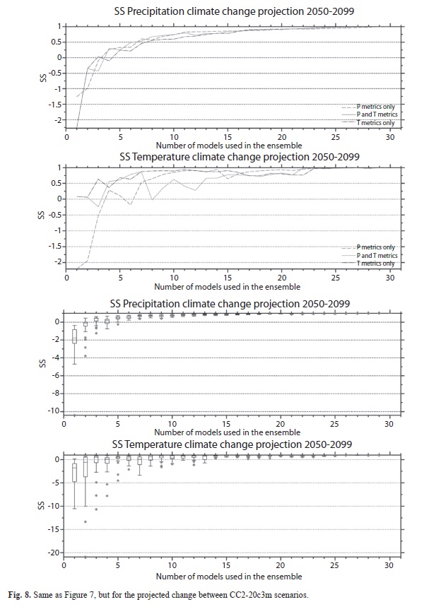
In this section we are interested in determining whether the nr values obtained previously in Parts I and II result in similar projected precipitation and temperature change for two climate change horizons: CC1 (2000 to 2049) and CC2 (2050 to 2099). The difference in the mean January to December future conditions (CC1 or CC2) and the 20c3m “historical” scenarios were computed for the same ensembles determined in Figure 4 and Figure 6 (See Brekke et al. 2008 for a discussion on how the climate change variable to be used affects the results). The SSs between the climate change patterns of each individual n-member ensemble and the MMEN for the two climate change horizons are shown in Figures 7 and 8. For the CC1 climate change horizon (and for the precipitation and temperature metrics), precipitation ensembles using the selection based on performance is positive (and stays positive) at around n=ncc1=6. In other words, the ensemble of 6 models (or more) is needed in order to guarantee that there is some skill in reproducing the climate change pattern of the MMEN. This also implies that the most conservative number of models used to create the ensemble between nr=7 and ncc1=6 would ensure that 1) the best performance of the model in reproducing the features of the “historical” period as shown in the Reanalysis is found and 2) the ensemble also has some skill in reproducing the same climate projection using as basis the ensemble of all available simulations. As can be seen both numbers of models are very similar and with n=7 the maximum skill in reproducing 20th century climate is found, along with some skill in reproducing the climate change patterns of the MMEN. In the case of precipitation random sampling, all the simulations have SSs greater than zero at n=ncc1=8, while the less conservative value of nr=7 found in Part II suggests that the constraint of having some skill in reproducing the climate change of the MMEN is more conservative. Note that the normalized Euclidean distances shown on figures 4 and 6, do not say anything about the absolute distances and therefore both figures are not comparable to each other. But in Figures 7 and 8, the use of the Skill Score (Equation 1) to test the similarity between the projected climate of the MMEn and MMEN allow comparison between the charts for any single climatic parameter (precipitation or temperature) and climate change scenario.
In the case of temperature, the creation of ensembles using the performance criteria suggests that n=ncc1=13 is needed (point where solid line is positive and stays positive in second panel from the top in Figure 7) in order to obtain positive SS values, contrasting with the n=nr=7 found in Part I of the analysis. This suggests that if the sampling is based on performance criteria, the ensemble of the best 13 models are needed in order to guarantee some skill in reproducing the climate change patterns of the multi-model ensemble, and that the maximum skill is achieved. In the case of random sampling, n=ncc1=15 is needed, in contrast with n=nr=6 found before. In Table 2 a summary of the results is presented for both climate change horizons. The results are very similar and support the same conclusions discussed in this part of the analysis.
Discussion
When selecting a subset of simulations and/or models for a regional study, it is very common to use some performance criteria to determine which simulations to use. Consistent with other studies, it was found here, that the selection and the results are very sensitive to the metrics used to rank the simulations. In this study, this multi-model ensemble of all available simulations was used as a benchmark to compare the results of the climate change simulations with the objective of determining if using a smaller subset of simulations results in very different climate projections.
The results showed that culling the models based on performance criteria or on random sampling, results in future precipitation projections that have some similarity to the projections obtained from the MMEN. For temperature, more models are needed to be added to the ensemble to guarantee skill in reproducing climate change patterns of the MMEN. It could be argued that the use of the MMEN as a benchmark is not justified as it contains models with very low skill in reproducing observations, but it is assumed here that as more simulations are included in the ensemble, the more noise is going to be filtered out and therefore this benchmark has superior characteristic than the multi-model ensemble of a subset of n<N simulations or MMEn.
Among other aspects discussed here, this assumption depends also on the sensitivity of the models in the area of study and the parameter used. This particular area showed low sensitivity (in particular to precipitation) when the skill of individual models were computed (Fig. 2). Moreover the region also shows no clear and consistent trend in precipitation means during the projected 21st century climate (Maldonado & Alfaro 2011, Hidalgo & Alfaro 2012), although it does show an evident warming tendency (Hidalgo & Alfaro 2012). Studies in other regions may provide more information regarding the size of the ensembles needed in other cases.
Conclusion
The inclusion of models in the multi-model ensemble based on their rank of reproducing 20th century climate showed great variability depending on which type of metrics were used to determine their rank. For the precipitation variable, ranks based on precipitation and temperature metrics (solid curve of top panel of Figure 4) showed that inclusion of models reach a maximum skill (lowest ΔSS/ΔSSmax) at around 7 models. When the models are introduced at random we found that around that same number of models the maximum skill is found. Therefore it seems that the inclusion of around 7 models out of 30 is the optimum number of models to produce an ensemble if the ranks are based on precipitation and temperature metrics. Note that it is not suggested that the 7 models culled according to their rank or selected at random have the same absolute skill; it only means that beyond 7 models there is not much change in the skill (or actually there is a degradation of the skill caused by models that do not contribute to improve the overall skill of the MMEn). If we use temperature metrics to determine the rank of the models for the precipitation variable (dark dash dotted line of top Figure 4), the maximum skill is found at the MMEN. It is difficult to interpret what this means in terms of the distribution of the skill of the MMEn. For the temperature variable, if we use precipitation and temperature metrics (solid curves of bottom Figure 4), when we reach 7 models there is a point of maximum skill (lowest ΔSS/ΔSSmax) and then the skill changes slightly until the 30 models are introduced in the MMEN. This is the same than the 7 randomly selected models that can be combined to reach the plateau in skill in Figure 6. When the precipitation patterns are used to determine the ranks of the models to be used to compute the skill for the temperature variable, the maximum skill is reach at around 21 models (light dashed line of bottom Figure 4). It can be concluded from all this that in general there is an optimum number of models/ simulations to be used in the ensemble and that number could be significantly lower than the total number of models/simulations. However, finding this optimum number is difficult as it is heavily dependent on how the models are introduced into the multi-model ensemble and on the type of metrics used. This however, does not guarantee that the climate change patterns produced by the MMEn are similar to the patterns produced by the MMEN as this has to be determined in a separate analysis.
Acknowledgments
This work was partially financed by projects (808-A9-180, 805-A9-224, 805-A9-532, 808-B0-092, 805-A9-742, 805-A8-606 and 808-A9-070) from the Center for Geophysical Research (CIGEFI) and the Marine Science and Limnology Research Center (CIMAR) of the University of Costa Rica (UCR). Thanks for the logistics support of the School of Physics of UCR. The authors were also funded through an Award from Florida Ice and Farm Company (Amador, Alfaro and Hidalgo). HH is also funded through a grant from the Panamerican Institute of Geography and History (GEOF.02.2011). The authors are obliged to André Stahl from UCR who processed much of the raw GCM data and Mary Tyree from Scripps Institution of Oceanography who provided the land-sea masks of the models. Also to María Fernanda Padilla and Natalie Mora for their help with the data base. Finally, to the National Council of Public University Presidents (CONARE), for the support of a FEES project “Interacciones oceáno-atmósfera y la biodiversidad marina del Parque Nacional Isla del Coco” (project 808-B0-654, UCR). We would like to thank two anonymous reviewers and Dr. Javier Soley that helped improve the quality of this article.
References
Alfaro, E. 2008. Ciclo diario y anual de variables troposféricas y oceánicas en la Isla del Coco, Costa Rica. Rev. Biol. Trop. 56 (Supl. 2): 19-29. [ Links ]
Amador, J.A. & E.J. Alfaro. 2009. Métodos de reducción de escala: Aplicaciones al tiempo, clima, variabilidad climática y cambio climático. Rev. Iberoamer. Econ. Ecol. 11: 39-52. [ Links ]
Barnett, T., D.W. Pierce, H. Hidalgo, C. Bonfils, B.D. Santer, T. Das, G. Bala, A.W. Wood, T. Nazawa, A. Mirin, D. Cayan, & M. Dettinger, 2008, Human-induced changes in the hydrology of the western United States. Science 319: 1080-1083. [ Links ]
Brekke, L.D., M.D. Dettinger, E.P. Maurer & M. Anderson. 2008. Significance of model credibility in estimating climate projection distributions for regional hydro- climatological risk assessments. Clim. Change 89: 371-394. [ Links ]
Cayan, D.R., E.P. Maurer, M.D. Dettinger, M. Tyree & K. Hayhoe. 2008. Climate change scenarios for the California region. Clim. Change 87: S21-S42. [ Links ]
Cortés, J. 2008. Historia de la investigación marina de la Isla del Coco, Costa Rica. Rev. Biol. Trop. 56 (Supl. 2): 1-18. [ Links ]
Guinde S. V. & J.A.N. Noronha. 2012, Design of IRR filters (last visit: July 4th, 2012, available at http://www.ee.vt.edu/~jnoronha/dsp_proj2_report.pdf). [ Links ]
Henderson, S., A.M. Rodríguez & R. McManus. 2008. A new future for marine conservation. Eastern Tropical Pacific Seascape. Technical Document: 4 p. (last visit: May 6th, 2010, available at http://www.conservation.org/). [ Links ]
Hidalgo, H.G., & E.J. Alfaro. 2012. Some physical and socio-economic aspects of climate change in Central America. Prog. Phys. Geog. 36: 379-399. [ Links ]
Hidalgo, H.G., T. Das, M.D. Dettinger, D.R. Cayan, D.W. Pierce, T.P. Barnett, G. Bala, A. Mirin, A.W. Wood, C. Bonfils, B.D. Santer & T. Nozawa. 2009. Detection and attribution of streamflow timing changes to Climate Change in the Western United States. J. Clim. 22: 3838-3855. [ Links ]
IPCC. 2010. The Intergovernmental Panel on Climate Change. The IPCC Data Distribution Centre. Available at http://www.ipcc-data.org/. Accessed January to July 2010. [ Links ]
Israel G.D. 2009. Determining Sample Size. University of Florida Institute of Food and Agricultural Sciences (IFAS) Extension publication. PEOD6. 7 pp. [ Links ]
Kalnay, E., M. Kanamitsu, R. Kistler, W. Collins, D. Deaven, L. Gandin, M. Iredell, S. Saha, G. White, J. Woollen, Y. Zhu, A. Leetmaa & R. Reynolds. 1996. The NCEP/NCAR 40-Year Reanalysis Project. Bull. Amer. Meteor. Soc. 77: 437-471. [ Links ]
Maldonado, T. & E. Alfaro. 2011. Revisión y comparación de escenarios de cambio climático para el Parque Nacional Isla del Coco, Costa Rica. Rev. Biol. Trop. This volume. [ Links ]
Maurer, E.P. & H.G. Hidalgo. 2008. Utility of daily vs. monthly large-scale climate data: an intercomparison of two statistical downscaling methods. Hydrol. Earth Syst. Sci. 12: 551-563. [ Links ]
Meehl G.A., C. Covey, T. Delworth, M. Latif, B. McAvaney, J. F. B. Mitchel, R.J. Stouffer & K.E. Taylor. 2007. The WRCP CMIP3 multimodel dataset. Bulletin of the American Meteorological Society. DOI:10.1175/BAMS-88-9-1383: 1383-1394. [ Links ]
PCMDI. 2010. Lawrence Livermore National Laboratory Program for Climate Model Diagnosis and Intercomparison. Available at http://www-pcmdi.llnl.gov/. Accessed August 2009 to July 2010. [ Links ]
Pierce D.W., T.P. Barnett, H.G. Hidalgo. T. Das, C. Bonfils, B. Sander, G. Bala, M. Dettinger, D. Cayan & A. Mirin. 2008. Attribution of declining western US snowpack to human effects. J. Clim, 21: 6425-6444. [ Links ]
Pierce, D.W., T.P. Barnett, B.D. Santer & P.J. Gleckler. 2009. Selecting global climate models for regional climate change studies. Proc. Nat. Acad. Sci. USA 106: 8441-8446. [ Links ]
Quirós-Badilla, E. & E. Alfaro. 2009. Algunos aspectos relacionados con la variabilidad climática en la Isla del Coco, Costa Rica. Rev. Clim. 9: 33-34. [ Links ]
Spiegel, M. 1998. Estadística. Serie Shaum. 2da ed. McGraw-Hill, México D.F., México. 556 p. [ Links ]
*Corespondencia: Hugo G. Hidalgo: Escuela de Física, Universidad de Costa Rica, 11501-2060 San José, Costa Rica; hugo.hidalgo@ucr.ac.cr. Centro de Investigaciones Geofísicas, Universidad de Costa Rica, 11501-2060 San José, Costa Rica.
Eric J. Alfaro: Escuela de Física, Universidad de Costa Rica, 11501-2060 San José, Costa Rica; erick.alfaro@ucr.ac.cr. Centro de Investigaciones Geofísicas, Universidad de Costa Rica, 11501-2060 San José, Costa Rica. Centro de Investigación en Ciencias del Mar y Limnología, Universidad de Costa Rica, 11501-2060, San José, Costa Rica.
1. Escuela de Física, Universidad de Costa Rica, 11501-2060 San José, Costa Rica; hugo.hidalgo@ucr.ac.cr, erick.alfaro@ucr.ac.cr..
2. Centro de Investigaciones Geofísicas, Universidad de Costa Rica, 11501-2060 San José, Costa Rica.
3. Centro de Investigación en Ciencias del Mar y Limnología, Universidad de Costa Rica, 11501-2060, San José, Costa Rica.
Received 29-IX-2010. Corrected 16-VII-2012. Accepted 24-IX-2012.

