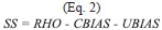
]]>
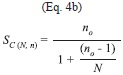
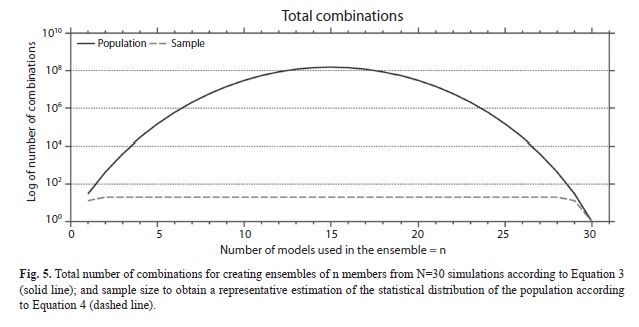
where “ceil” is the rounding to the higher integer, Z2 is the abscissa of the normal curve that cuts off an area at the tails (1-confidence level, e.g. 95%), p is equal to the estimate proportion that is present in the population, while the value of q is given by q=1-p. Since p has an unknown aspect, the most conservative option for p and q (p=q=0.5) was used as it produces the ]]>
no value. Also e=0.05 is the error that is anticipated to be committed. Inspection of the equation showed that it converges to a plateau very rapidly (Fig. 5). Equation 4 was tested using a Monte Carlo simulation for ensembles of sizes n=1 to n=6. The SS distributions for the populations were computed, and 100 000 samples of ]]>
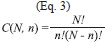
C(N,n) combinations of n simulations were computed. The samples and the population distributions were compared using a Kolmogorov–Smirnov or K–S test. It was verified that the error committed was below 5% and therefore this serves as an indication that Equation 4 gives useful estimations of the needed sample size. Selection of model ensembles
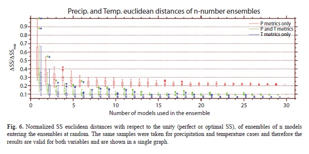
In Figure 6 the results for the random selection of simulations are shown. The same samples were selected for precipitation and temperature and therefore the results for both variables are the same in Figure 6. At around n=nr=7 there is ]]>
ΔSS/ΔSSmax, suggesting that the inclusion of more models at random does not substantially improve the skill beyond that point. ]]>
Part III Implication for climate change projections In this section we are interested ]]>
Figure 4 and Figure 6 (See Brekke et al. 2008 for a discussion on how the climate change variable to be used affects the results). The SSs between the climate change patterns of each ]]>
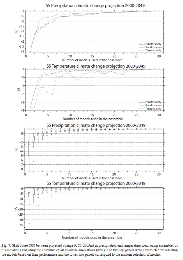
N for the two climate change horizons are shown in Figures 7 and 8. For the CC1 climate change horizon (and for the precipitation and temperature metrics), precipitation ensembles using the selection based on performance is positive (and stays positive) at around n=ncc1=6. In other words, the ensemble of 6 models (or more) is needed in order to guarantee that there is some skill in reproducing the climate change pattern of the ]]>
N. This also implies that the most conservative number of models used to create the ensemble between nr=7 and ncc1=6 would ensure that 1) the best performance of the model in reproducing the features of the “historical” period as shown in the Reanalysis is found and 2) the ensemble also has some skill in reproducing the same climate projection using as basis the ensemble of all available simulations. As can be seen both numbers of models are very similar and with n=7 the maximum skill in reproducing 20th century climate is found, along with some ]]>
N. In the case of precipitation random sampling, all the simulations have SSs greater than zero at n=ncc1=8, while the less conservative value of nr=7 found in Part II suggests that the constraint of having some skill in reproducing the climate change of the MMEN is more conservative. Note that the normalized Euclidean distances shown on figures 4 and 6, ]]>
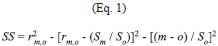
absolute distances and therefore both figures are not comparable to each other. But in Figures 7 and 8, the use of the Skill Score (Equation 1) to test the similarity between the projected climate of the MMEn and MMEN allow comparison between the charts for any single climatic parameter (precipitation or temperature) and climate change scenario.
In the case of temperature, the creation of ensembles using the performance criteria suggests that n=ncc1=13 is needed (point where solid line is positive and stays positive in second panel from the top in Figure 7) in order to obtain positive SS values, contrasting with the n=nr=7 found in Part I of the ]]>
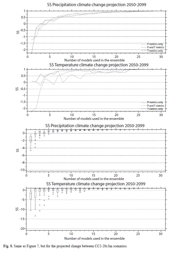
Table 2 a summary of the results is presented for both climate change horizons. The results are very similar and support the same conclusions discussed in this part of the analysis.
]]>
Discussion When selecting a subset of simulations and/or models for a regional study, it is very common to use some performance criteria to determine which simulations to use. Consistent with other studies, it was found here, that the selection ]]>
The results showed that culling the models based on performance criteria or on random sampling, results in ]]>
N. For temperature, more models are needed to be added to the ensemble to guarantee skill in reproducing climate change patterns of the MMEN. It could be argued that the use of the MMEN as a benchmark is not justified as it contains models with very low skill in reproducing observations, but it is assumed here that as more simulations are included in the ensemble, the more noise is going to be filtered out and therefore this benchmark has superior ]]>
n. Among other aspects discussed here, this assumption depends also on the sensitivity of the models in the area of study and the parameter used. This particular area showed low sensitivity (in particular to precipitation) when the skill of individual models were computed (
Fig. 2). Moreover the region also shows no clear and consistent trend in precipitation means during the projected 21st century climate (Maldonado & Alfaro 2011, Hidalgo & Alfaro 2012), although it does show an evident warming tendency (Hidalgo & Alfaro 2012). Studies in other regions may provide more information regarding the size of the ensembles needed in other cases. ]]>
Conclusion The inclusion of models in the multi-model ensemble based on their rank of reproducing 20th century climate showed great variability depending on which type of metrics were used to determine their rank. ]]>
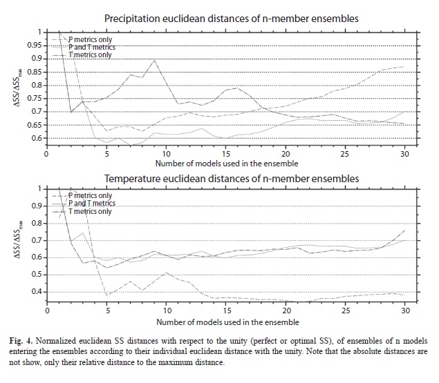
Figure 4) showed that inclusion of models reach a maximum skill (lowest ΔSS/Δ
SSmax) at around 7 models. When the models are introduced at random we found that around that same number of models the maximum skill is found. Therefore it seems that the inclusion of around 7 models out of 30 is the optimum number of models to produce an ensemble if the ranks are based on precipitation and temperature metrics. Note that it is not suggested that the 7 models culled according to their rank or selected at random have the same absolute skill; it only means that beyond 7 models there is not much change in the skill (or actually there is a degradation of the skill caused by models that do not ]]>
n). If we use temperature metrics to determine the rank of the models for the precipitation variable (dark dash dotted line of top Figure 4), the maximum skill is found at the MMEN. It is difficult to interpret what this means in terms of the distribution of the skill of the MMEn. For the temperature variable, if we use precipitation and temperature ]]>
Figure 4), when we reach 7 models there is a point of maximum skill (lowest ΔSS/ΔSSmax) and then the skill changes slightly until the 30 models are introduced in the MMEN. This is the same than the 7 randomly selected models that can be combined to reach the plateau in skill in
Figure 6. When the precipitation patterns are used to determine the ranks of the models to be used to compute the skill for the temperature variable, the maximum skill is reach at around 21 models (light dashed line of bottom Figure 4). It can be concluded from all this that in general there is an optimum number of models/ simulations to be used in the ensemble and that number could be significantly lower than the total number of models/simulations. However, finding this optimum number is difficult as it is heavily ]]>
n are similar to the patterns produced by the MMEN as this has to be determined in a separate analysis. Acknowledgments
This work was partially financed by projects (808-A9-180, 805-A9-224, 805-A9-532, 808-B0-092, 805-A9-742, 805-A8-606 and 808-A9-070) from the Center for Geophysical Research (CIGEFI) and the Marine Science and Limnology Research Center (CIMAR) of the University of Costa Rica (UCR). Thanks for the logistics support of the School of Physics of UCR. The authors were also funded through an Award ]]>
References Alfaro, E. 2008. Ciclo diario y anual de variables troposféricas y oceánicas en la Isla del Coco, Costa Rica. Rev. Biol. Trop. 56 (Supl. 2): 19-29. [ Links ] Amador, J.A. & E.J. Alfaro. 2009. Métodos de reducción de escala: Aplicaciones al tiempo, clima, variabilidad climática y cambio climático. Rev. Iberoamer. Econ. Ecol. 11: 39-52. [ Links ] Barnett, T., D.W. Pierce, H. Hidalgo, C. Bonfils, B.D. Santer, T. Das, G. Bala, A.W. Wood, T. Nazawa, A. Mirin, D. Cayan, & M. Dettinger, 2008, Human-induced changes in the hydrology of the western United States. Science 319: 1080-1083. [ Links ] Brekke, L.D., M.D. Dettinger, E.P. Maurer & M. Anderson. 2008. Significance of model credibility in estimating climate projection distributions for regional hydro- climatological risk assessments. Clim. Change 89: 371-394. [ Links ] Cayan, D.R., E.P. Maurer, M.D. Dettinger, M. Tyree & K. Hayhoe. 2008. Climate change scenarios for the California region. Clim. Change 87: S21-S42. [ Links ] Cortés, J. 2008. Historia de la investigación marina de la Isla del Coco, Costa Rica. Rev. Biol. Trop. 56 (Supl. 2): 1-18. [ Links ] Guinde S. V. & J.A.N. Noronha. 2012, Design of IRR filters (last visit: July 4th, 2012, available at http://www.ee.vt.edu/~jnoronha/dsp_proj2_report.pdf). [ Links ] Henderson, S., A.M. Rodríguez & R. McManus. 2008. A new future for marine conservation. Eastern Tropical Pacific Seascape. Technical Document: 4 p. (last visit: May 6th, 2010, available at http://www.conservation.org/). [ Links ] Hidalgo, H.G., & E.J. Alfaro. 2012. Some physical and socio-economic aspects of climate change in Central America. Prog. Phys. Geog. 36: 379-399. [ Links ] Hidalgo, H.G., T. Das, M.D. Dettinger, D.R. Cayan, D.W. Pierce, T.P. Barnett, G. Bala, A. Mirin, A.W. Wood, C. Bonfils, B.D. Santer & T. Nozawa. 2009. Detection and attribution of streamflow timing changes to Climate Change in the Western United States. J. Clim. 22: 3838-3855. [ Links ] IPCC. 2010. The Intergovernmental Panel on Climate Change. The IPCC Data Distribution Centre. Available at http://www.ipcc-data.org/. Accessed January to July 2010. [ Links ] Israel G.D. 2009. Determining Sample Size. University of Florida Institute of Food and Agricultural Sciences (IFAS) Extension publication. PEOD6. 7 pp. [ Links ] Kalnay, E., M. Kanamitsu, R. Kistler, W. Collins, D. Deaven, L. Gandin, M. Iredell, S. Saha, G. White, J. Woollen, Y. Zhu, A. Leetmaa & R. Reynolds. 1996. The NCEP/NCAR 40-Year Reanalysis Project. Bull. Amer. Meteor. Soc. 77: 437-471. [ Links ] Maldonado, T. & E. Alfaro. 2011. Revisión y comparación de escenarios de cambio climático para el Parque Nacional Isla del Coco, Costa Rica. Rev. Biol. Trop. This volume. [ Links ] Maurer, E.P. & H.G. Hidalgo. 2008. Utility of daily vs. monthly large-scale climate data: an intercomparison of two statistical downscaling methods. Hydrol. Earth Syst. Sci. 12: 551-563. [ Links ] Meehl G.A., C. Covey, T. Delworth, M. Latif, B. McAvaney, J. F. B. Mitchel, R.J. Stouffer & K.E. Taylor. 2007. The WRCP CMIP3 multimodel dataset. Bulletin of the American Meteorological Society. DOI:10.1175/BAMS-88-9-1383: 1383-1394. [ Links ] PCMDI. 2010. Lawrence Livermore National Laboratory Program for Climate Model Diagnosis and Intercomparison. Available at http://www-pcmdi.llnl.gov/. Accessed August 2009 to July 2010. [ Links ] Pierce D.W., T.P. Barnett, H.G. Hidalgo. T. Das, C. Bonfils, B. Sander, G. Bala, M. Dettinger, D. Cayan & A. Mirin. 2008. Attribution of declining western US snowpack to human effects. J. Clim, 21: 6425-6444. [ Links ] Pierce, D.W., T.P. Barnett, B.D. Santer & P.J. Gleckler. 2009. Selecting global climate models for regional climate change studies. Proc. Nat. Acad. Sci. USA 106: 8441-8446. [ Links ] Quirós-Badilla, E. & E. Alfaro. 2009. Algunos aspectos relacionados con la variabilidad climática en la Isla del Coco, Costa Rica. Rev. Clim. 9: 33-34. [ Links ] Spiegel, M. 1998. Estadística. Serie Shaum. 2da ed. McGraw-Hill, México D.F., México. 556 p. [ Links ]
*Corespondencia: Hugo G. Hidalgo: Escuela de Física, Universidad de Costa Rica, 11501-2060 San José, Costa Rica; hugo.hidalgo@ucr.ac.cr. Centro de Investigaciones Geofísicas, Universidad de Costa Rica, 11501-2060 San José, Costa Rica.
Eric J. Alfaro: Escuela de Física, Universidad de Costa Rica, 11501-2060 San José, Costa Rica; erick.alfaro@ucr.ac.cr. Centro de Investigaciones Geofísicas, Universidad de Costa Rica, 11501-2060 San José, Costa Rica. Centro de Investigación en Ciencias del Mar y Limnología, Universidad de Costa Rica, 11501-2060, San José, Costa Rica.
1. Escuela de Física, Universidad de Costa Rica, 11501-2060 San José, Costa Rica; hugo.hidalgo@ucr.ac.cr, erick.alfaro@ucr.ac.cr.. 2. Centro de Investigaciones Geofísicas, Universidad de Costa Rica, 11501-2060 San José, Costa Rica. 3. Centro de Investigación en Ciencias del Mar y Limnología, Universidad de Costa Rica, 11501-2060, San José, Costa Rica. ]]>
Received 29-IX-2010. Corrected 16-VII-2012. Accepted 24-IX-2012.
