


 Inglés (pdf)
 Articulo en XML
 Referencias del artículo
 Enviar articulo por email
 Citado por SciELO
  Similares en
SciELO
Similares en
SciELO 
 Permalink
Introduction
Every day, countless systems of all kinds interact with each other in an ecosystem that is invisible to the inexperienced eye, these systems generate large amounts of information that other systems take advantage of, these can be both natural and artificial. In many cases, the data does not appear to be directly related, however, all of this data is grouped into groups of information that exceed the logic of natural deduction, since they can be in different groups and states at the same time.
Human-made systems are not always in the appropriate form, so when a system needs to be migrated or upgraded, a lot of time can be wasted on its understanding, which leads to great losses of time and money. Viewing systems as graphs can reduce understanding time and facilitate optimization.
The main objective of this article is to illustrate how second order systems can be converted into graphics, through a representative technique, for their understanding and subsequent normalization, while having secondary objectives such as providing a support tool for analyze complex systems of diverse nature and show the relationship between Armstrong's axioms, graph theory and second-order logic.
Background
Two great precedents of this work are W. Armstrong axioms, which has been applied since its publication until today for the normalization of relational databases, through the inference of functional dependencies, the other is set theory, a fundamental pillar of the Structured Query Language (SQL), for daily use by countless computer systems worldwide, which was designed to manage and retrieve information.
Graphs have a lot of applications in information systems, in fact, there are very interesting works on graph theory such as Kumar, Raj, & Dharanipragada (2017), where heterogeneous graphs are analyzed to calculate using user-defined aggregate functions; or in the work of Ren, Schneider, Ovsjanikov, & Wonka (2017), that make groupings through graphs to design joint graphs to visualize segmented mesh collections; or Shi et al. (2017) where to combine contextual social graphs.
At the database level there are a couple of jobs where they normalize databases, one is Frisendal, T. (2020) where normalize database schemas using graphs, in a very simple way, without the need to add additional elements to the language, however it is different since It represents a different mechanism of using graphs to normalize a database, it does not establish mechanisms to break loops within graphs, presenting limitations regarding reciprocity, on the other hand, the way to use edges is node to node (1: 1), while the one shown here allows to group and separate the nodes as convenient with the creation of compound nodes, second is the work of Attallah, B. (2017) where It uses interactive visualization tools to normalize databases, although it is effective for human understanding and analysis, it presents multiple differences with respect to the current work, since it has an approach to solve while playing instead of working with graphs.
However, the way of using the graphs in this article has not been used before, basically due to the high complexity of the initial graph and the way to seek the simplification of problems through sometimes complex abstractions, not complex from normalization, but from the visualization.
Justification
This method aims to provide an alternative way to solve the problems resulting from complexity, it does not attempt in any way to replace existing models, but rather to be a support tool. Being a visual method, it can be easier to understand and solve, supporting both professionals and students, since more algebraic methods are currently taught and used, this method attempts to offer a more natural technique.
At an academic level, the article opens a debate on the best way to teach and present the topic of systems normalization in general (including databases). It is also proposed that these methods could be automated, since the proposed compound graph structures can be easily modeled as data structures in algorithms in programming languages (as with the object-oriented programming paradigm) and the different types of dependencies to delete could be detected as patterns or cycles.
Context
The current work emerged as an idea in a database course at the University of Costa Rica in 2015, after seeing the professor normalize a relational database, the idea was "this procedure is slow and complicated, it can be simplified by drawing "After weeks of analysis the foundations of the current work were created, however, other teachers could not understand it, despite being a functional work, on the other hand, it did not have sufficient mathematical foundation to formalize. In 2019, as Engineer and with more mathematical knowledge, he continues the development of this work. This work is born from a humble family and at no time has financial support been received from any kind for the preparation of it, however the university is thanked for the education received.
Theoretical reference
This work has three main references, they are the theory of graphs, Armstrong's Axioms and second order logic, the latter is vital to understand the multilevel structure of graphs, since functional dependencies can be denoted as elements of Second order.
Graph theory.
Graph theory is a branch of mathematics, widely used in computing, that studies graphs and their properties. Graphs (usually represented by the letter 'G') are made up of a set of points called "nodes" or "vertices", represented by the letter "V" and a set of "edges" or "arcs" represented by the letter 'E', where each edge is in charge of joining two or more vertices, therefore a graph can be expressed as G = (V, E), in some cases the graphs have more than one set of vertices.
Armstrong's Axioms.
Armstrong's axioms are a set of rules to infer restrictions between the relationships that exist in a relational database, which are called functional dependencies and whose set is denoted by the letter F, so we can see the Axioms of Armstrong of the form R 𝑈 , 𝐹 , where U are the attributes of the schema and R the function that relates the attributes.
Methodology
Approach
The current work has a qualitative approach, since it has a problem of interest with respect to functional dependencies and the observation of the new properties that are obtained when applied them to subsystems. The scope is explanatory, because, it is tried to demonstrate by means of the axioms and the existing theories, sometimes determining the whole as an axiomatic system.
Analysis units
Theoretical models of relational databases were studied, on occasions databases of my own design were selected, mainly to develop the logical basis, on other occasions they were randomly selected from free Internet exercises created for students, to carry out verifications of results. Only relational databases were used, since by their nature the applied demonstrations are more evident, the selection criteria were randomization.
Collection techniques
The technique of data collection was through experimentation and observation, focusing on pattern detection and cycle breaking, sometimes trial and error, checking each result against Armstrong's axioms, to retest.
Analysis Processing
Then multiple tests and checks to detect patterns and break cycles, a new general review of not contradicting Armstrong's Axioms was made, the result graphs were grouped in a categorical system and examined by second order logic, the result could not contradict the logic of first or second order. Each result can be demonstrated, however, most of the time they are reduced to common sense, fulfilling one of its objectives, simplicity.
Results
The data is the basis of the systems, a space where these are most evident are the databases and from the principles of their normalization and the theory of the graphs, focused on a system of systems, this concept of normalization of the Graph is born of graphs.
According to Bondy & Murty (1976), a graph can be displayed as 𝑉 𝐺 , 𝐸 𝐺 , 𝜓 𝐺 , where 𝑉 𝐺 is a non-empty set, 𝐸 𝐺 a disjoint set, with borders and 𝜓 𝐺 association functions. At the database level, we can be interpreting this association functions as functional dependencies (DF). In this technique only 𝑉 𝐺 and 𝜓 𝐺 are of interest, simplifying 𝑉 𝐺 , 𝑉 𝐺 , 𝜓 𝐺 as 𝑉 𝐺 , 𝜓 𝐺 , this definition is particularly convenient, since it coincides with the form of Armstrong's relational schema 𝑅 𝑋 , 𝐹 where, according to Armstrong, Nakamura, & Rudnicki(2002) “Let X be a set and let F be a non-empty dependency set of X. We see that the element of F is a dependency of X.”.
The way to operate this technique is breaking cycles (which we can see as redundancies) and detecting patterns to facilitate the simplification of the systems, these patterns are nothing more than the same dependencies, but on a larger scale, either because they have more nodes in a section or because they are displayed on groups of nodes instead of simple nodes. In some cases, it is necessary to normalize, but in others it is not, a normalized graph is easier to understand and in computational aspects it requires much less space for its storage, however, it complicates the query operations for having the more segmented information. In order to land the article, it will focus on the following points, mainly on how to normalize a database using graphs.
Representation
The final result of the representation of a non-standardized system is a graph of graphs, but when normalizing it, it is visualized as a graph of "nodes" (not necessarily 𝑛 0 ), to understand this better each attribute must be taken as a node and not as a chart, this means that a normalized table is equivalent to a simple graph.
The objective of normalization is to reduce relations to the maximum, having the same objective as a file compressor in a computer, in relation to the above it can be said that this is equivalent to the space occupied in the secondary memory.
In a database, all the attributes of a table can be seen as a node, but each one is different, so it is necessary to put a label, which is usually a letter, however, it often happens that in reality two attributes are a single element.
Advantages of using graphs
The success of normalizing using graphs resides in being visual, here are some advantages of them.
Types of relationships
First, it is necessary to define simple nodes as those of order 𝑛 0 and compounds such as those of order 𝑛 𝑥 , being able to see them in various ways.
The relationships between nodes can be classified into three types depending on their nature, which depend exclusively on the types of nodes involved. You can name the relationship types as point-to-point, dynamic, or interplanar.
Point to point
They are the typical connections that are made in each directed graph, basically consists of connecting two or more simple nodes, I call them that way by relating nodes of order 0 ( 𝑛 0 ). These are equivalent to one-to-one relationships of the databases. These point-to-point relationships and the output dynamics are those that are attempted at the time of normalization because they represent the lowest levels of complexity. They are of the form 𝜓 𝐺 : 𝐴→𝐵 .
Dynamics
If there are relations of a compound node with a simple one, it can be said that they are dynamic relationships, they are more common than they seem and in some cases of maximum normalization they remain in the solution. They are equivalent to one-to-many relationships and their detrimental complexity is slightly greater than point-to-point, but much less than interplanar.
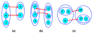
Interplanar
They are the product of interactions between subsystems, it occurs when there are two compounds and their internal nodes (individual or compound) are related. It can be called a pure interplanar relationship when the relationship is mediated by nodes of order 0, an exponential interplanar is similar to the previous one, but more internal (subsystems within the subsystem), finally, the dynamic interplanar is the one that relates a simple node and compound node.
If it is seen from a logical second order approach, we can define these relationships as those existing between the attributes of different objects, these relationships are semantically accepted, infrequent in natural language, but they appear frequently in systems, so we must be kept it in mind. Each relationship between planes is equivalent to a many-to-many relationship and represent a great unnecessary complexity in the system, so it should be avoided at all costs. Figure 1 illustrates the above.
Harmful dependencies
There are several types of relationships due to their unnecessary complexity, they contribute a lot of noise and inefficiency to the systems, very often they are the product of interactions between compound nodes (nodes that contain others inside) and simple nodes (points), although they can also happen between a single set of simple nodes.
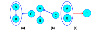
Reciprocal dependencies
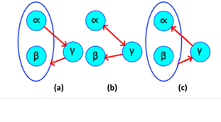
These dependencies arise from relations between simple and compound nodes, are simple to understand, as its name implies, is a type of relationship that returns to its origin, but in a compound way. They are functional when the origin goes from point to point and returns dynamically. A reciprocal relationship is illustrated in Figure 2.
Source: Own elaboration, 2020
Figure 2 (a) Reciprocal dependence; (b) Normal dependence. (c) Normal graph.
In this case the simple nodes contained in the compound are not directly related to each other, but it is known that {α→β, β→αλ}, as every node contains itself the dependence remains {α↔β, β→λ}. In essence it may seem easy step but tends to be confused with irreducible relationships as in Figure 2.C. If this is decomposed, we obtain {α→β, β→α, β→λ}, then with the union axiom the result is {α↔β, β → λ}.
In this case (αλ → β, β → α}) cannot be further reduced because there is no certainty of who defines {β} and there are no direct relations between {α, λ}, therefore it is said that is already normalized to the maximum possible. An easy way to distinguish reciprocal dependencies from non-reciprocal dependencies is by looking at their origin and destination, reciprocals start from a simple node and end up in a complex, the normal ones have the opposite direction (explained later in this article).
Association or associative dependencies
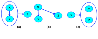
It is possible to affirm that the reciprocal relations of association in databases are associative in terms of subgroup relations and commutative in terms of the ends of the same relationship, the union axiom of Armstrong is equivalent to an relation association since {X → Y, XY → Z} = {X → YZ}, by what is said that what can be associated is only the nodes that travel in equal directions (same origin or same destination), never different because it causes loss of information. The commutation is simpler still, it is based on the principle of reflexivity that indicates that {X ← Y} ↔ {Y → X} and that {X → YZ} = {X → ZY}. This normalization can be tested using Armstrong's transitivity and union axioms.
With this being clear, it should be emphasized that the unnecessary complexity of a compound node will always be greater than that of a single node, hence the need to eliminate these relationships as much as possible. The Figure 3 illustrates what has been said.
Source: Own elaboration, 2020
Figure 3 (a) Associative dependence; (b) Normal dependency; (c) Normal dependence.
Given a relation defined as 𝜓 𝐺 := {X→Y, XY→Z}, it is determined that S is a associative relation, so a term must be eliminated from the relation {XY → Z} and no There is certainty of who directly defines {Z}, it must be eliminated to the smaller term ({Y}), since if it is related to {Z}, then by axiom of transitivity, so will {X }, But if {X} defines {A} there is no evidence that {Y} also does, so the relationship is defined by 𝜓 𝐺 :={X→Y, X→Z}. From Armstrong's point of view {X → Y, XY → Z} can be decomposed into {X → Y, Y → Z, X → Z}, if we eliminate {X → Z} no information is lost because by transitivity this relationship is deductible.
An easy way to conclude this by means of graphs, instead of with algebra, is to fix the relations of a compound node with a simple one, if in the compound all of its nodes are related to each other (it does not include the nodes of possible nodes Compounds within the compound), the nodes that can be candidate keys within the local system (within that composite node), will be those that relate to the simple node, therefore the composite node will become smaller. This is exemplified in Figure 4.
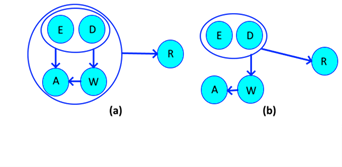
The largest will always be the one that is related to the outside, to determine the largest node (s) you only have to follow the arrows in the opposite direction until you cannot continue without leaving the local system
Redundancies
Many times, a set C of relationships tend to fall into redundancy, it could be said that in humans it functions as a mechanism that ensures that a message is transmitted, but in the machines in most cases, especially in databases, Is only an expense of resources.
There are two basic types, depending on the complexity of the interaction of all their relationships, since the major determinant of the nature of redundancies are the relationships and as has been said before these are translated in size and complexity. Redundancies are classified as Coupled and Cyclical.
Coupling
This type of redundancy has the same impact as that of cyclical, although visually they are very different, it is possible to move from one to the other through the axiom of additivity, however, the priority at this time is to know how to simplify them, for this it is enough with forming a linear relationship between the simple node and the root of the composite node. Figure 5.a shows a redundant dependency and 5.b shows normalization. In this case, if we decompose the expression we obtain {C→A,C→B,A→B}, isolating the subset {C→A,A→B} we can deduce by transitivity {C→B}, so that we can discard the latter dependency.
These relationships are very similar to association redundancies at the visual level, but their main difference is that these are not distributive, since their result is aligned, it can form a straight line. They differ visually from the association redundancies by the direction of their outermost point-to-point relationship.
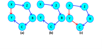
Cyclical
They are called so because the arrows form a circle, giving the intuition that the system rotates, although these cases do not cause drastic effects, it is important to eliminate them to have a complete optimization. These problems of redundancy can be determined by observing a graph, if a cycle is formed, there is almost certainly one of these cases. Let 𝜓 𝐺 = {X→Z, Z→B, B→C, C→Y, X→Y}, it follows that {X → Y} by transitivity, so it is not necessary to put that relation (see Figure 6)
Irreducible expressions
In some cases, if proper attention is not paid, mistakes can be made with irreducible expressions. This section tries to clarify these circumstances.
Indiscernible origin
In some cases, a relationship cannot be decomposed due to its high level of uncertainty regarding its origin, since if we isolate the subsystem the properties of the left sides of the equation are the same. Take for example {AB -> C} as a result of which the following unknowns arise: A -> C? B-> C? Or only together do they determine the relationship? Under this scenario the properties (P) of A and B are the same, representing itself as ∀𝐴∀𝐵 ∀𝑃(𝑃𝐴↔𝑃𝐵)→(𝐴=𝐵) . An example of these relationships is illustrated in Figure 1.C.
False cyclical
Understanding what is explained in the cyclical dependencies section, if there is more than one consecutive relationship in the opposite direction, then the set of relationships cannot be reduced, since they can be seen as 2 different paths that converge at the same point; On the other hand, if there is no relationship in the opposite direction to the others, then none can be eliminated without losing information to the system.
Recommended Algorithm
The steps used by each person to solve a problem are usually different, not that they are wrong, but there are sequences that can help solve the same problem in a better way. The following is an optimal three-step algorithm to solve the normalization by hand.
Case Study
Are 𝑉 𝐺 := {A, B, C, D, E, F, G, H} ^ 𝜓 𝐺 := {ABC→E, FD→A, AG→E, D→C, BC→F, A→H, F→D, H→G}; the graph formed by 𝜓 𝐺 → 𝑉 𝐺 is denoted by GE and is of the form (see Figure 7a).
First associative relationship removed (see figures 7b and 7c).
Second associative relationship eliminated (see figure 7d).
Cyclical dependency eliminated, since BC→A ^ A→A ABC→E (figure 7e).
Alignment (optional) (see figure 7f).
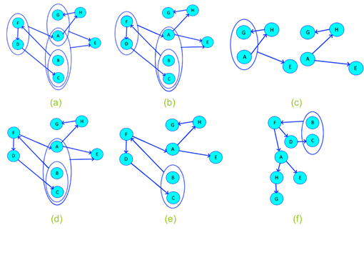
Source: Own elaboration, 2020
Figure 7 Case study:(a) Initial state; (b) first associative relationship removed; (c) first associative on detail; (d) second associative relationship removed; (e) Cyclical dependency eliminated; (f) Alignment (optional).
As you can see, it went from a highly complex system, full of reciprocal, associative and redundant relationships to an almost linear system, in four steps, without losing information related to its functional dependencies, if it is verified algebraically, we can see that the same result is achieved.
Are 𝑉 𝐺 := {A, B, C, D, E, F, G, H} ^ 𝜓 𝐺 := {ABC→E, FD→A, AG→E, D→C, BC→F, A→H, F→D, H→G}.
Order
ABC→E, FD→A, AG→E, BC→F, F→D, D→C, A→H, H→G
Redundancy is eliminated by transitivity
A→H ^ H→G ^ AG→E ( A→G ( A→E
ABC→E, FD→A, A→E, BC→F, F→D, D→C, A→H, H→G
F→D ^ FD→A ( F→D ^ F→A
ABC→E, F→A, A→E, BC→F, F→D, D→C, A→H, H→G
Redundancy is eliminated by transitivity
BC→F ^ F→A ^ A→E ( ABC→E
F→A, A→E, BC→F, F→D, D→C, A→H, H→G
Conclusions
Usually people are reluctant to make a chart whose nodes are other charts, it seems like a very complicated idea and with few practical uses, however this article shows the opposite. The simplicity of the way of operation makes the technique repeatable by anyone, since it is simply based on the breaking of cycles and the detection of patterns. This method of system normalization is humanely easier to analyze and solve problems that can be drawn on paper than those expressed through mathematical abstractions.
The hypothesis of this work was to demonstrate whether it is possible to create an axiomatic system for the simplification of complex systems through such a natural method as drawing the system to be analyzed in graphs, which respect Armstrong's axioms, considering qualifiers for subsets or properties; it is evident through this method arising from database techniques, but it is easily applicable to other areas, while it has a high analytical power and various forms of use, its use depending mainly on the nature of the problem.
These methods are compatible with computational data structures, which could allow their coding to create systems that automate the analysis, also through symbol manipulation (rewriting systems). After knowing how to trace the problem, the only thing that is a little complicated is identifying the reciprocal, associative and redundant relationships, but with some exercises it is very easy to learn.
Personally, this method worked very well for me as a student, it is a visual alternative, but it has great potential. When it comes to applying across multiple fields, maybe it just takes a little creativity to find amazing apps.

