


 English (pdf)
 Article in xml format
 Article references
 Send this article by e-mail
 Cited by SciELO
  Similars in
SciELO
Similars in
SciELO 
 Permalink
1. Introduction
According to the World Health Organization (WHO) (2020) ''homicide is the killing of a person by another with intent to cause death or serious injury, by any means. It excludes death due to legal intervention and operations of war”. Unfortunately, since 2006, when the Mexican government started a frontal war against organized crime, both violence and homicides rates have increased. That is why we consider that analysing homicide mortality through Machine Learning (ML) and Statistical Design of Experiments (DOE) can contribute to the definition of strategies and actions to reduce incidence of this kind of crime in Mexico. Statistics about the severity of insecurity in Mexico are available in Observatorio Nacional Ciudadano (2015, 2016 and 2017).
In accordance with United Nations Office on Drugs and Crime (UNODC) (2019), just considering intentional homicides (related to interpersonal conflict, or criminal activities or, sociopolitical agendas) in 2017, the average global homicides rate was 6.1 per 100,000 people around the world and 17.2 in the Americas region. It also reported that, Central America and South America were the sub-regions with the highest homicides rates (25.9 and 24.2, respectively). The top homicide rates correspond to El Salvador with 62.1 and Venezuela with 56.8.
Although the rate for the Mexican case was around half of Venezuela's, the most impressive thing is how it has grown. In fact, according to the National Institute of Statistics and Geography (INEGI) in 2017, there were 32,079 homicides that implied a rate 26.0, which is 3.6 times the figure reported ten years ago with 8,867 cases and a rate 8.1 (INEGI, 2019). Even worse, 2017 preliminary figures from the INEGI (2018) indicate that states such as Colima and Baja California Sur have very high homicide rates (113 and 91 respectively).
It is worth saying that these states have reported homicide rates higher than the above-mentioned countries. These statistics are in line with the violent environment that exists in the country, which is recognized by the Mexican Ministry of the Interior: approximately 40,000 people missing, more than 1,100 hidden burial sites and around 26,000 unidentified bodies in the forensic services . Nowadays, the homicide related violence in Mexico is concentrated in six states that account for 60 % of all homicides in the country: Chihuahua, Baja California, Guerrero, Sinaloa, Nuevo León, and Tamaulipas.
The 2019 Mexico Peace Index (Institute for Economics and Peace, 2020) points out that peace has deteriorated in 2018. In fact, the national homicide rate increased by 14% in 2018. Mexico's funding for justice is half of the OECD average; furthermore, it is notorious how 97% of crimes go unpunished. The state of Yucatán is the most peaceful state, while Baja California is the least peaceful one. Guanajuato and California Sur recorded the largest deterioration and the largest improvement respectively in their peace scores. This index depends on homicides rates, the target variable to model in this paper.
Zepeda and Jimenez (2019) established based on official information that 2018 was the most violent year ever recorded, given that every 15 minutes a person was killed, reaching more than 33 thousand homicides. The authors also confirm that there is a decline in convictions for this crime, resulting in high rates of impunity. In this sense, Guerra (2020) reported that 9 out of 10 serious crimes such as homicides go unpunished, although he views this as an optimistic perspective since some homicides are not reported. In general, this social phenomenon appears to be an upward spiral of deaths and impunity. One of the most direct consequences of increasing homicides in demographic terms is the decrease in life expectancy (González et al., 2012; Aburto et al., 2016) or its not increasing (Ordorica-Mellado & Cervantes-Salas, 2021).
The objective of this work is to identify some sociodemographic and economic factors to explain homicide mortality. This will be achieved using several statistical learning methods taking into account only quantifiable information at hand, comparing them, and selecting the best method and identify key factors influencing homicides. Once we determine a final model, we will focus only on those factors that we consider that can be influenced in the medium term by changes in Mexican public policy and estimate their effect on the homicide rate with the use of a two-level fractional factorial design. The target variable in our approach is homicide, which takes the values of one when the cause of death corresponds to codes X85-Y09 and Y87, reported in the International Classification of Diseases (ICD-10), taken from the WHO (2015), and takes the value of zero otherwise.
2. Literature Review
Rodríguez (2016), by means of the approach called the ''extremely violent societies'' examines the nature of the violence in Mexico, where the changes in type of violence and the participation of different actors over the analysed period are considered. The author exposes a series of violent behaviours that coexists together in Mexico. Among his main findings are that the government actions to fight violence have been unsuccessful and ineffective. Conforming to Díaz (2016), few theories or evidence help us understand a homicide's dynamic in Mexico. Likewise, he takes a tour through different theories and states that inequality is one of the most consistent findings in the criminological literature, which relates economic situation and homicides. Then he uses regression models and suggests that to have a good explanation of homicides, an indicator of poverty and inequality should be included as an independent variable.
Hernández et al. (2018), through a comparative longitudinal study analysed mortality associated with violence. They state that violence can be decoded as a significant public health problem, with consequences that affect all kinds of people. They add that Mexico has recently presented a critical increase associated with drug trafficking. In fact, between 2006 and 2011, it was up 150 %, where the main victims were economically active men. They also point out the need to improve police, fight impunity and corruption, as well as strengthen the justice system. Likewise, Quimet et al. (2018), show that low levels of social control (poor law enforcement, corruption and an inefficient and ineffective justice system) lead to higher murder rates.
Medina and Villegas (2019), focused on homicides in the younger population, from 10 to 24 years old. Using Poisson regression, they found that homicides are significantly associated with unemployment of the population over 12 years of age, households made up of people who are not relatives, low school attendance and income below the welfare line. They suggest establishing inter-sectoral policies to reduce inequality gaps, achieve better living conditions, well-being levels and providing health services to people and their communities.
Arteaga et al. (2019), focus on the spatial correlation of homicides and the places where criminal bands operate. The authors also comment that the criminal bands in some cases act as enemies, while in others, they collaborate. Their analysis is made at the municipal level in the years 2005, 2010 and 2015, and they prove the association between homicides and criminal bands' locations. In turn, McLean et al. (2019) establish a so-called ''neoliberalism-homicide hypothesis”. Through regression analysis, using two global measures of neoliberalism and information from 142 countries in 2014, they find that there is little evidence to support the cited hypothesis. Then they disaggregate the variables that make up these indexes and deduce that homicide rates increase when both, size of government and tax burden become more neoliberal. They conclude that neoliberal government policies suggest increasing poverty and inequality, which also implies increasing homicide rates.
A descriptive report about homicides in Mexico was presented by INEGI (2019). This document provides some characteristics about homicides to help understand the phenomenon during the 1990 to 2017 period. Some general results are the following: young people homicides involved an estimated loss of 17.6 million life years; most were young men with basic schooling and economically active; the main means used were firearms and sharps; and finally, it is very likely that homicides occur on weekends and in urban areas. Cadena and Garrocho (2019) also expose the dynamics of homicides in Mexico, geographically speaking from 2006 to 2017, incorporating forced disappearances to their description. In their essay, the authors discover spatial patterns that are useful in identifying priority regions. Thereby, the statistical relationship at the municipal level between homicides and forced disappearances is analysed.
An interesting point of view is addressed through the so-called spread of homicides at a geographical level (INEGI, 2019). Furthermore, Gamlin and Hawkes (2017) argue that death from homicides follows epidemic levels for the Mexican case. The authors also compare it to that experienced in some countries that have similar socioeconomic development and conclude that it is one of the worst. They also study a historical exploration of political economy, masculinity and violence. In another context, Zeoli et al. (2012) had described a similar approach, where, in agreement with the authors, homicides could be understood as an infectious disease. In that study, the spatial and temporal homicide's dynamic at Newark, New Jersey is illustrated. Additionally, a spatial-temporal propagation pattern was identified and so was the population vulnerable to this cause of death.
More recently, there have been some research papers that have focused on application of ML methods to mortality. For instance, in order to obtain accurate mortality forecasting, Levantesi and Nigri (2019) propose a method based on the combination of Random Forest and a two-dimensional P-spline. That model accuracy is evaluated, and its impact is measured on contracts, considering several countries and the Lee–Carter model. Likewise, Nigri et al. (2019) define a ''Lee–Carter model family'' and suggest a new approach to model the future trend of mortality behaviour through a Recurrent Neural Network with a long short-term memory architecture that produces improvements in terms of predictive accuracy.
From a holistic perspective, Levantesi et al. (2020) present the main results of the current actuarial literature about the potential of ML and their drawbacks in predicting mortality and improving the longevity risk quantification and management on life products. Thereby, they point that the ML methods improve both fitting and forecasting of the traditional models. Perla et al. (2021) show how the structure of the Lee–Carter model can be generalized using a simple shallow convolutional network model. In fact, they also show that their proposal has some benefits such as an enhanced predictive performance over deep networks and highly accurate forecasts. Finally, Nigri et al (2021) propose a new approach for forecasting life expectancy and lifespan disparity based on recurrent neural networks with a long short-term memory. Their results are compared to projections taken from different models and seem to be coherent, reasonable, and more accurate. Likewise, in this case, Vital Mortality Statistics (VMS) is used in conjunction with other sociodemographic, economic, social and public indicators from this underdeveloped country that is paradoxically placed at the top six tourist world destinations (World Tourism Organization (UNWTO], 2018).
3. Materials and methods
3.1 Data sources
It is important to emphasize that the UNODC recognizes the quality of the Mexican homicide data as good[3]. These data consist of 2,673,887 observations from 2014 to 2017. Additionally, it was necessary to make the following assumptions to make the subsequent estimates:
1.Sociodemographic information on the marginalization index is the same for the years under the scope of the study, and there are no significant differences between the actual number of homicides and those reported in the INEGI statistics by the entities. Although a recognizable difference exists, it is believed to be systematic and similar throughout the entities during the period under study.
2.Gender alert and the other variables are constantly maintained for all entities during the period; the quality of reported homicides is the same in all states in the country.
New variables were created to include information regarding the current state of violence and insecurity. Particularly, a variable was created to reflect information related to what is called Gender alert. This mechanism has emerged due to the violence against women. This variable was defined as 1 for every state that has a Gender alert, and 0 otherwise, based on the National Women's Institute. The states that have at least one municipality declared with Gender alert by year are, according to the National Women's Institute, 2020: a) State of Mexico and Morelos in 2015; b) Michoacán, Nuevo Leon, Veracruz and Chiapas in 2016; c) Sinaloa, Colima, San Luis Potosí, Guerrero, Quintana Roo and Nayarit in 2017.
According to the Instituto Mexicano de la Competitividad (IMCO) (2018), the Rule of Law Index (RLI) is a global instrument that looks at the Rule of Law comprehensively. It consists of eight factors further disaggregated into 44 sub-factors; the eight factors followed by their number of subfactors (in parenthesis) are: constraints on government powers (6), absence of corruption (4), open government (4), fundamental rights (8), order and security (3), regulatory enforcement (5), civil justice (7) and criminal justice (7). Among the sub-factors that are obviously related with this paper are: effective control of crime, the right to life and security of the person is effectively guaranteed, people can access and afford civil justice, criminal investigation system is effective and criminal adjudication system is timely and effective. The RLI is built from results taken from applied surveys to citizens, lawyers and experts.
In accordance with IMCO (2018a), the Corruption Index (CI) is a perception taken from experts and businesspeople about public sector corruption. In fact, Mexico's CI is at the same level of those of countries such as Guinea, Iran and Russia. In the report, it is argued that the decline of basic political rights in México, is one of the principal causes why the corruption in Mexico is limited. Among some suggestions made for Mexico in order to improve its score, is to eradicate impunity by closing the gap between anti-corruption legislation and its application.
México Evalúa (2018), stablishes that the Criminal Justice System Maturity measures whether the states are able to implement integral public policies focused on strategic planning processes, as well as follow-up mechanisms and an efficient resource management system. Thereby, it indicates if the Criminal Justice System has the necessary elements required in order to have the institutional capabilities and the ability provide suitable results in the prosecution and administration of justice.
The sociodemographic marginalization index (CONAPO, 2016), is a linear combination of the following factors: total population in 2015; % of illiterate population 15 years or older; % of the population 15 years or older with incomplete elementary education; % of occupants of households with neither drainage nor toilets; % of occupants of households without electricity; % of occupants of households without tap water; % of households with some level of overcrowding; % of occupants of households with dirt floor; % of the population in places with less than 5,000 inhabitants; % of the population employed with incomes up to two minimum wages. It is worth mentioning that minimum wage changed in the analysis period (ranging from approximately 124 to about 154 US dollars per month). The distribution of municipalities according to this index is (from more to less marginalization): 283 (11.5%), 817 (33.3%), 514 (20.9%), 498 (20.3%) and 345 (14%). Also, some variables from the Consejo Nacional de Evaluación (CONEVAL) (2018) and the US Department of State-Bureau of Consular Affairs (2018) were taken into account. In summary, the variables considered are listed in Table 1.
Table 1 Description of used variables.
| Variable (Label) | Value | Source |
| Homicide (homi) | 1-Homicide, 2-Not homicide | INEGI |
| Sex (Sex) | 1-Men, 2-Women, 9-Missing | INEGI |
| Victim's age (Age) | 0-100 | INEGI |
| Age group (Age_group) | 1- less 1 year, 2- 1 year, ,,,, 5- four years, 6- 5 to 9 years,…, 28 – 115 to 119 years, 29 - 120 years, 30 - Missing. | INEGI |
| Highest education level achieved (high_edu) | 1-No schooling, 2-10: Kindergarten: Graduate School | INEGI |
| Economic activity at time of death (eaatd) | 1-Yes, 2 & 8-No, 9-Missing | INEGI |
| Type of job/occupation (job) | 1:9- From Managers to Blue collar, 10,11, 97-Do not work, 98 & 99 - Missing. | INEGI |
| Season when occurred (season_occur) | 1:4-Winter: Fall, 99-Missing | INEGI |
| Victim lived alone or not (alone) | 1-Alone, 2-With couple, 9-Missing | INEGI |
| Time of occurrence (hour_occur) | 1-Night, 2-Morning, 3-Afternoon, 4-Evening | INEGI |
| Month of occurrence (moc) | 1-12, 99-Missing | INEGI |
| Nationality (nationality) | 1-Mexican, 2-Foreigner, 9-Missing | INEGI |
| Native language other than Spanish (dialect) | 1-Yes, 2-No, 9-Missing | INEGI |
| Urban area (urban_area) | 1-Urban, 2-Rural, 9-Missing | INEGI |
| Population in place of residence (spr) | 1:5-From smallest to largest, 99-Missing | INEGI |
| Population in place of occurrence (spo) | 1:5-From smallest to Largest, 99-Missing | INEGI |
| Margination index (MI) | 1-Highest, 2-High, 3-Medium, 4-Low, 5-Lowest | CONAPO |
| GINI (GINI) | 0-1 | CONEVAL |
| Criminal justice system maturity (CCJSI) | 0-1000 (see Section 3.1) | México Evalúa |
| Population in preventive prison (PPP) | 0-1x100000 | México Evalúa |
| Rule of Law Index (RLI) | 0-1 (see Section 3.1) | IMCO |
| Corruption Index (CI) | 0-1 (see Section 3.1) | IMCO |
| Mexico travel advisory (MTA) | 1-Normal precautions, …, 4-Do not travel | US Department |
| Gender alert (GA) for state of residence (ga_ent_resid) | 1-State with GA, 2-State without GA | NWI |
| Gender alert (GA) for state of occurrence (ga_ent_ocurr) | 1-State with GA, 2-State without GA | NWI |
| % Pop. in moderate poverty (MPoverty) | Percentage (0-100%) | CONEVAL |
| % Pop. in extreme poverty (EPoverty) | Percentage (0-100%) | CONEVAL |
| % Pop. with moderate food insecurity (PPMFI) | Percentage (0-100%) | CONEVAL |
| % Pop. with severe food insecurity (PPSFI) | Percentage (0-100%) | CONEVAL |
| % Pop. with lag in education (PPLE) | Percentage (0-100%) | CONEVAL |
| % Pop. without health services (PPWHS) | Percentage (0-100%) | CONEVAL |
| % Pop with limited health services (PPWLHS) | Percentage (0-100%) | CONEVAL |
| % Pop. 65+ without soc. security (P65WASS) | Percentage (0-100%) | CONEVAL |
3.2 Data limitations
It is important to recognize the limitations of the data employed in this work and point out that there are other sources not considered here. Among these, there are official sources such as The Executive Secretariat of the National Public Security System (SESNSP) (2015a, 2015b, 2016, 2017), and non-official, like those coming from the Mexican newspaper Milenio, or a map of homicides elaborated by an activist. However, there is not enough information about the victims; in general, only the total number of homicides is available. It should be noticed that the VMS does not report homicide classifications such as intentional homicide, killings in self-defense, killing in legal interventions or non-intentional homicide (for details see UNODC, 2019).
We should also note that we could not consider other factors that contribute to homicides in Mexico, since they are either non-public or unquantifiable, or both (at state or municipal or individual level). For instance: (a) an index that reflects the flux of guns from the United States to Mexico through the so-called "Fast and Furious" agreement from 2006; (b) empirical evidence of the possible association between politicians and criminals, (c) quantifiable features about criminal groups and (d) drug trafficking and drug consumption. We recognize that our paper just tries to explore the phenomenon with public and quantifiable information at hand using a statistical perspective.
Overall, there is no relevant information available about some of the victims' conditions like income, heritage, bank account, use of credit cards, number of children, workplace, leisure activities and so on. Information is also limited concerning the murderer such as family conditions, parental violence, parental drug or alcohol abuse, absence of parents, economic situation of his/her family, his/her criminal or psychological record, educational level, etcetera. It is also important to say that we do not pretend to show any formal theory about homicides using the Mexican case, but we just want to present results obtained from a statistical approach.
3.3 Methods
Our approach relies on ML and DOE methods. Since for each observation in our data set, we have an associated response, which is either homicide or non-homicide, we are dealing with supervised learning in the case where the response is categorical and we are trying to ''learn'' a function that relates the input factors with the response.
Given that cause of death is recorded for each of the deaths reported in VMS, we approached the identification of key factors influencing death by homicide from a classification perspective, as a supervised learning problem, having two possible outcomes, either the cause of death was homicide, or it was not. From the classification perspective, ''homicide”, is the class of interest or positive class, meanwhile ''not homicide'' is the negative class. It should be noted that this homicide identification in the dataset is equivalent to that of the WHO mentioned above (WHO 2015). Thereby, the target variable was recoded as 1 if the case corresponds to homicide, and 0 otherwise. Then, a three-step approach followed in this work is: 1.- Select the best classification model, 2.- Model tuning and variability assessment and 3.- Apply a DOE considering key factors influencing homicide incidence. Model fitting was done in the statistical software R version 4.1.0 (R Core Team, 2021). The caret package written by Kuhn (2020), short for classification and regression training, was used for model selection and tuning. Prior to modelling, data was pre-processed to eliminate highly correlated and near zero variance predictors.
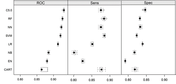
Given the significant unbalance in the data since less than 3.62% of the deaths in the dataset were homicides, the accuracy is not appropriate as a criterion to select a model to predict homicides. That is why, we use the area under the Receiving Operating Characteristic (ROC) curve as the selection criterion (Fawcett, 2006). This criterion considers the sensitivity, that is, the model's ability to correctly identify actual homicides (true positive rate), and the specificity, which is the ability to correctly identify the cases that were not homicides (true negative rate). The area under the ROC curve is denoted by AUC, although in the figures, it is identified as ROC.
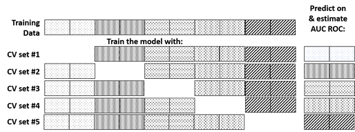
We split the data in a training set (70%) and a test set (30%), ensuring that the proportion of homicides was the same in both sets as in the original full data set, using then only the training set for model selection. Five-fold cross-validation repeated five times was used to estimate the quality measure, associated with a given ML method to evaluate its performance (model selection), and to select the appropriate level of complexity (model tuning). The folds and repetition subsets were set before model training, thus, ensuring that each algorithm uses the same data partitions and repeats to achieve a fair comparison.
In general, K-fold cross-validation (CV) involves randomly dividing the set of observations in K groups of approximately the same size. One of the folds is treated as a validation set (test set) and the other (K-1) folds are used to train the model; the procedure is repeated for each of the K folds, resulting in K estimates of the AUC, similar to Fujita et al. (2016), to evaluate the validity of our model. The process is repeated R times, hence obtaining KR estimates of the area under the ROC curve for each of the models included in the analysis. Five-fold cross-validation is illustrated in Figure 1. It is important to mention that Molinaro (2005) and Kim (2009) showed that repeating K-fold cross-validation increases the precision of the estimates, thereby maintaining a small bias.
Furthermore, given the high level of unbalance present in the data, prior to training each model for each fold and repetition, the training subset was balanced. There are two commonly used methods to balance the data, the first being oversampling the minority class so that in the training subset, there is almost equal representation of the minority class (homicide) and the majority class (not homicide). The second method, which is the one applied in this work, was to under-sample the majority class in the training set, so that there is almost equal representation of the majority and minority classes in the training subset. Whether under-sampling or over-sampling is used, this is only done on the training subset and not in the validation subset.
We compare eight different statistical classification methods for our analysis, for details we suggest see the cited references. Two linear models: Logistic Regression (Agresti, 2002) and Elastic Net (Friedman et al., 2010). Three non-linear models: Neural Networks (Bishop, 2009), Support Vector Machines (Cortes and Vapnik, 1995; Vapnik, 1996) and Naïve Bayes (Rish, 2001). And finally, three classification algorithms: CART (Shannon, 1948, Breiman et al., 1984, Therneau and Atkinson, 2019), C5.0 (Quinlan, 1992; Kuhn and Johnson, 2013, Kuhn and Quinlan 2018) and Random Forest (Breiman, 2001).
4. Results
4.1 Model selection
As a first step, we compared the models pointed above. Our prioritization is based on empirical instead of statistical criteria such as the one proposed by Bengio and Grandvalet (2004) and Bouckaert (2004). Considering only the ROC criteria, the best model was the rule model based on the C5.0 algorithm, followed by the Random Forest as can be seen in Figure 2.
4.2 Model tuning
As a second step, once the C5.0 algorithm was selected, instead of using a 70/30 mix for training and testing, data was split into training (80 %) and test (20 %) sets to carry out fine tuning of the model (Alberg, 2015, June 14). Given the significant imbalance present in the data, the 80/20 percent split was done utilizing stratified sampling to ensure that in both, the training set and test set, the proportion of homicides was approximately 3.62 %. Given this class unbalance, as done during the model selection stage, training for each fold and repetition, was done down-balancing the data in the subset used for training, so that the number of observations belonging to both classes were approximately the same. The tuning parameters were the number of boosting iterations (trials), with or without variable selection (winnow) and tree or rules. The objective of the tuning process is to maximize the area under the ROC curve.
The tuning grid consisted of 25, 50, 75 and 100 trials, variable selection (yes / no) and type of model (tree/rules) yielding a total of 16 combinations of the hyperparameters. The ten-fold cross-validation procedure is repeated 3 times, resulting in 30 estimates of the area under the ROC curve for each of the 16 combinations of the tuning parameters. This process led us to a best model with 100 boosting iterations (trials), without variable selection and rules generation. Since this final model provided 30 estimates of the area under the curve, these were used to assess its variability, yielding a mean AUC of 93.14% (sd 0.16 %); a sensitivity of 85.00% (sd 0.37 %); and specificity of 88.32% (sd 0.52 %). The overall results are shown in Figure 3, while the top ten results are shown in Table 2.
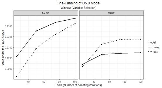
Table 2 Cross-validation results for C5.0 model tuning.
| Model Type | Variable Selection (winnow) | Trials | ROC (%) | Sensitivity (%) | Specificity (%) | ROCSD (%) | SensSD (%) | SpecSD (%) |
| rules | FALSE | 100 | 93.14 | 85.00 | 88.32 | 0.16 | 0.37 | 0.52 |
| rules | FALSE | 75 | 93.12 | 84.85 | 88.43 | 0.15 | 0.37 | 0.54 |
| tree | FALSE | 100 | 93.11 | 84.68 | 88.54 | 0.13 | 0.11 | 0.29 |
| rules | FALSE | 50 | 93.08 | 84.88 | 88.33 | 0.14 | 0.34 | 0.56 |
| tree | FALSE | 75 | 93.06 | 84.80 | 88.38 | 0.14 | 0.12 | 0.32 |
| tree | TRUE | 100 | 93.04 | 84.43 | 88.71 | 0.16 | 0.31 | 0.52 |
| tree | TRUE | 75 | 93.04 | 84.46 | 88.69 | 0.15 | 0.33 | 0.51 |
| tree | TRUE | 50 | 93.01 | 84.49 | 88.61 | 0.15 | 0.37 | 0.56 |
| tree | FALSE | 50 | 92.99 | 84.74 | 88.32 | 0.14 | 0.15 | 0.34 |
| rules | TRUE | 100 | 92.98 | 84.69 | 88.28 | 0.19 | 0.56 | 0.72 |
Note:ROCSD, SensSD and SpecSD are the standard deviations of the area under the ROC curve, the sensitivity and specificity, respectively.
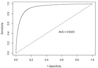
The final model was then used to predict homicides in the test data set (20 % of the complete data set). The results are presented in the Confusion Matrix in Table 3, and the ROC curve is presented in Figure 4. The following statistics were obtained: AUC 93.23 %, accuracy 85.00 %, sensitivity 88.73 % and specificity 84.86 %.
Table 3 Confusion matrix with test set (20%).
| - | Reference | ||
| Prediction | - | Not homicide | Homicide |
| Not homicide | 437,362 | 2,183 | |
| Homicide | 78,046 | 17,185 | |
4.3 DOE to Estimate the Effects of Key Factors Influencing Homicides
The third step in our approach is to estimate the effect of key factors influencing homicides. The factors in Figure 5 were found to be the most important factors in the final model.
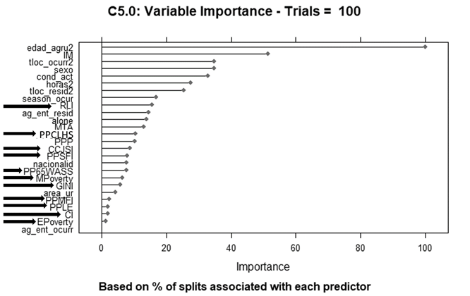
Figure 5 Factors marked with an arrow are those that can be influenced directly by changes in public policies and regulations.
Among the 26 most important factors, we selected those that can be influenced directly, by changes in public policy, laws and/or regulations, and to make recommendations on where efforts must be made to be able to significantly reduce homicide rates in Mexico. The selected factors (predictors), marked with arrows in Figure 5, together with their lowest and highest levels are presented in Table 4, where low and high levels correspond to the extremes of each indicator found in some states of the country.
Table 4 Selected factors that can be influenced by changes in public policies.
| Factors | Label | Low Level | High Level |
| Rule of Law Index | RLI | 0.29 | 0.45 |
| % Pop. with limited health services | PPCLHS | 9.10 | 22.80 |
| Criminal justice system maturity | CCJSI | 134.00 | 483.00 |
| % Pop. with severe food Insecurity | PPSFI | 4.30 | 23.90 |
| % Pop. 65 + without soc. security | PP65WASS | 5.20 | 23.10 |
| % Pop. in moderate poverty | MPoverty | 13.60 | 50.50 |
| GINI | GINI | 0.378 | 0.578 |
| % Pop. with moderate food insecurity | PPMFI | 7.20 | 21.40 |
| % Pop. with lag in education | PPLE | 8.40 | 29.00 |
| Corruption Index | CI | 0.27 | 0.42 |
| % Pop. in extreme poverty | EPoverty | 0.60 | 28.10 |
To assess how these factors can impact homicide rates through the predictive model, we designed a resolution V two level fractional factorial design in 128 runs denoted by 2_V^(11-4). Resolution V designs have the property that main effects are confounded with four factor interactions and two factor interactions are confounded with three factor interactions. The design was generated and its results analyzed with the FrF2 R package (Grömping, 2014). For a complete discussion of fractional factorial designs at two levels, the reader is referred to the classical book by Box et al. (1978).
For each factor, the low and high levels were set, respectively to the lowest and highest values for that factor in the country. We ran the 128 combinations with the optimized model, replacing the corresponding factors in all the observations by the levels indicated in the design, obtaining for each one of these 128 executions of the model, a predicted homicide rate at the country level. The values of the other variables remained unchanged from actuals in each of the runs.
After executing the 128 runs, the normal probability plot of the effects (Figure 6 (left)), showed that the only significant effects are: RLI, CCJSI, PP65WASS, GINI, PPLE, EPoverty and CI, as well as the interactions PPCLHS*CCJSI, and RLI*MPoverty and RLI*GINI.
After analyzing the effects and interaction plots, we concluded that, although they were statistically significant, the only effect with practical importance is the RLI. This is not only due to its large impact in magnitude, but also because this is an index that, with adequate public policies, can be directly impacted by its components linked with order and security as well as criminal justice. In other words, from our perspective, given a poor RLI, impunity emerges as an incentive for the continuous consummation of homicides in Mexico.
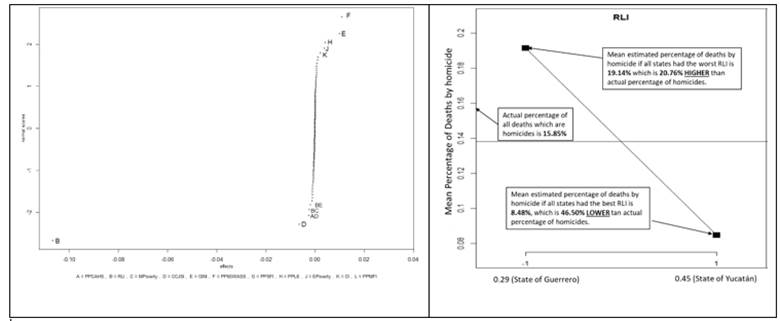
Figure 6 Normal probability plot of the effects (left) and Effect of the RLI on homicide incidence (right).
As shown in Figure 6 (right), if all states in Mexico had an RLI = 0.45 corresponding to the state of Yucatán, which is the best in the country, given that all other conditions remained the same, homicide rates could be reduced by up to 46.5 %. On the other hand, if all states in Mexico had an RLI as bad as the one for Guerrero, where RLI = 0.29, given all other conditions remained unchanged, homicide rates could increase by 20.8 %. Certainly not all the states in Mexico have an RLI as bad as that of Guerrero, so, if we assumed that all states had the median RLI of 0.37, moving them to an RLI such as the one for Yucatan, would reduce homicide rates by approximately 23.3 %, provided all other conditions remained without change. Therefore, a very important lever to reduce homicide rates in the country is to implement policies and procedures in all states to achieve a suitable RLI.
5. Conclusions
The C5.0 ML approach to identify the key variables looks the best. In fact, we consider that it is efficient and promising. The use of DOE proved to be very useful to determine that domestic changes in public policy, laws and regulations to improve the RLI, could lead to a significant reduction in homicide rates in Mexico. However, given the phenomenon's dynamic and complexity, we consider that it would be necessary to apply this class of models periodically and/or by region.
Our results are consistent with Díaz (2016) who states that inequality (which we can associate with GINI index), is one of the most consistent findings in the criminological literature, relating economic situation and homicides. The fact that RLI, CCJSI and CI are statistically significant is consistent with Hernández et al. (2018) and Quimet et al. (2018), who imply that high violence related mortality is associated with poor law enforcement, impunity, corruption and an ineffective justice system. Finally, statistical significance of interactions involving EPoverty, MPoverty and PPCLHS is consistent with results from McLean et al. (2019) which indicate that increasing poverty and inequality implies increasing homicide rates.
Our findings are also in line with some of Eisner's (2016) proposals. He makes some suggestions to reduce violence and related death rates by reducing corruption and bribery in all its forms; developing effective, accountable and transparent institutions at all levels; and promoting the RLI and equal access to justice. In accordance with our estimates, the RLI variable was the most important factor to predict homicides in the C5.0 model; moreover, it has the maximum impact to reduce homicides in Mexico according to the results of our DOE. In this sense, our findings are and will be marginal, until some off-the-record information becomes quantifiable and taken into account in conjunction with that utilized in this work.
The present results have some limitations. The homicides phenomenon is too diverse and dynamic in Mexico, that is why it requires a permanent analysis across time and space. For instance, homicide causes can be attributable, among others, to cultural, religious or political beliefs which can be very different in small communities, versus large cities, where the homicides are usually caused by armed robberies or kidnapping. Likewise, amid the COVID-19 pandemic homicides' trend has not have any changes despite the generalized lockdown. We expect that with more explicative factors at the municipal level, it could be possible to get a better understanding of phenomenon to formulate an appropriate intervention policy. Thereby, we can affirm that our results are valid for the period of time under consideration, however under different circumstances, like the pandemic or a serious economic crisis, other possible patterns may occur.

