Introduction

Conceptual hydrological models are important tools in operational hydrology, water resources planning and management. These models approximate the general physical mechanisms governing the hydrologic processes through simplified equations, which make them less demanding in terms of model input data and therefore more computationally efficient (¹). Nevertheless, due to their simplified structure, initial values of relevant parameters of conceptual models are usually unknown and must be estimated through calibration using suitable optimization algorithms (²). In general, optimization methods can be classified as either local or global based on their search strategies (³). Local methods rely on exploitation, which means that they are carried out by initialization of parameter sets and then iteratively minimizing the objective function; according to a set of deterministic rules. These rules direct the parameter search towards finer solutions. Exploitation may lead to high performance and faster convergence of the optimization method. Nonetheless, the decision on how to sample the following parameter space depends on previous samplings, which can cause the method to getting trapped in multiple local minima or promote premature convergence. Global methods on the other hand, rely on exploration, meaning that the optimization of the objective function is improved by randomly looking into different regions of the parameter space, while keeping the information learned from previous samplings. At the start of the optimization process, global methods largely explore the parameter space to subsequently converge into sub-regions that might contain the global minima based on the response surface type. This is done by a set of deterministic and statistical rules (⁴). Estimates from local optimization methods may considerably vary based the choice of starting parameter values (⁵). Global methods on the other hand can cope with multiple local minima, discontinuous derivatives and high dimensionality, but are considerably slower than local methods. This is particularly relevant when the evaluation of the cost function is expensive and only a limited number of evaluations are feasible. This somehow makes global methods less attractive in hydrological applications due to its elevated computational cost (⁶). Various studies have compared the application of global optimization methods in hydrological modelling using several model-structures and under different climatic conditions (^{7 : 9}). Nevertheless, an extensive comparison of local and global methods aimed to identify the pros and cons of each method in hydrological modelling has been mostly left aside. Relevant research questions include: How effective are global and local optimization methods for the calibration of a conceptual hydrological model?, How prone are global and local optimization methods to getting trapped in local minima based on different sets of initial model parameters? Does the duration of the calibration period significantly affect the performance of the various optimization methods and can shorter calibration periods be used confidently? Consequently, this study attempts to answer the abovementioned research questions through the calibration of the HBV-TEC conceptual hydrological model applied to a case study in Costa Rica.

Methodology

Study area and data sources.

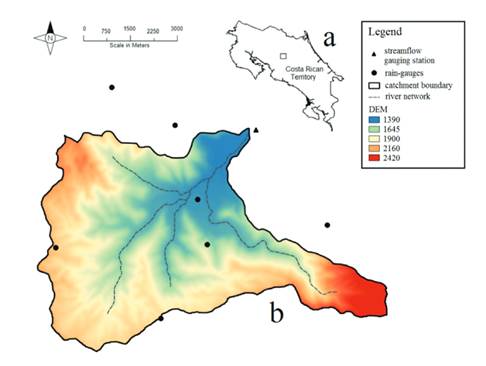
The upper Toro River catchment (43.15 km2) is located in the province of Alajuela in north-western Costa Rica (figure 1). The topography is mountainous with elevations ranging from 2593 to 1334 m. The slope is steep with a mean value of 23%. The mean annual rainfall of the area is 4200 mm and the mean annual temperature range is between 17.2 and 32.8 ºC. The land use in the catchment is dominated by forest (62%) and grassland (35%) with minor contributions from other uses; mainly water and urban. The catchment has a highly complex precipitation pattern and its temporal and spatial distribution is influenced by factors such as El Niño southern oscillation (ENOS), geomorphology, rugged terrain and microclimates. Rainfall and temperature were calculated from aggregated daily measurements at 8 rain-gauges (figure 1). Daily observed streamflow data for the same period were obtained from ICE-12-6 streamflow gauging station. The catchment boundary was delineated using a RapidEye 10 m digital elevation model (DEM). The monthly long-term mean potential evapotranspiration records were calculated using the Penman-Monteith method. Rainfall and temperature were calculated using a powered-3 inverse distance weighting (IDW) interpolation method.

Figure 1 (a) Position of the upper Toro River catchment in Costa Rica; (b) Upper Toro River catchment boundary, river network, RapidEye digital elevation model (DEM), rain-gauges and streamflow gauging station. 

The HBV-TEC hydrological model

In this study, the HBV-TEC hydrological model (¹⁰) was selected for its simplicity, local development, parsimony, robustness and ease of use. The HBV-TEC is a redesign of the HBV (Hydrologiska Byråns Vattenbalansavdelning) model (¹¹) developed using the R programming language (¹²). The HBV-TEC is a semi-distributed conceptual rainfall-runoff model for continuous calculation of runoff. The basic concept is that discharge is related to storage through a conservation of mass equation and a transformation routine. The hydrologic response is easily modelled due to the use of lumped/semi-distributed data and a simplified conceptual representation of flow processes. The structure of the HBV-TEC model consists of routines for precipitation, soil moisture, response function and transformation. The model can be run using daily or hourly time-steps; input data are precipitation, air temperature and long-term estimates of monthly potential evapotranspiration.

Optimization process and experimental design

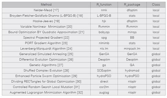
Eight global and eight local optimization methods were used in this study. All methods are currently implemented in R (table 1). The Nash-Sutcliffe efficiency (NSE) was selected as the objective function of the optimization process. For the purpose of this paper, NSE efficiency values over 0.75 are considered satisfactory. The NSE objective function is defined as:

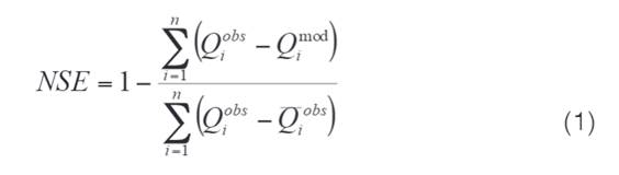
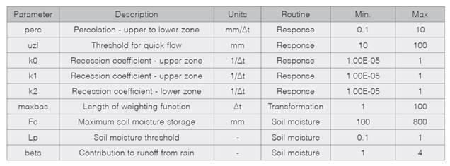
where i is the timestep, nis the total number of time-steps,wis relative weight assigned to each observation, Qis the discharge and subscriptsobsand modrefer to observed and modelled correspondingly. A total of nine HBV-TEC model parameters (perc, uzl, k0, k1, k2, maxbas, fc, lp and beta), which have a direct influence on runoff generation were considered. The chosen parameters control the total volume and shape of hydrographs and are associated with the response, routing and soil moisture routines of the model. Parameter optimization ranges (table 2) were selected based on recommended literature values (13:16). Additionally, optimization methods Differential Evolution Optimization (Deoptim), Genetic Algorithms (ga) and DIviding RECTangles Algorithm for Global Optimization (direct) do not include arguments for initial parameter values; on the contrary, only upper and lower parameter bounds of the cost function are considered. The experimental design was structured based on the abovementioned research questions. To increase the likelihood that the full parameter space could be sampled by all optimization methods, 50 sets of initial parameters were randomly sampled across the feasible parameter boundaries of the HBV-TEC model by fixing a reproducible seed. This allowed each optimization method to start with the same initial sets of parameters, sequentially organized from 1 to 50. Four different durations of the calibration period, 4, 8, 12 and 16 years (Y4, Y8, Y12 and Y16), were selected from historical records ranging from years 1994 to 2010. Termination criteria was based either on (a) relative convergence tolerance, where the optimization method stops if it is unable to reduce the value by a factor of relative tolerance, which defaults to sqrt(CPU-precision), in this case 1e-6 or (b) or maximum number of function evaluations allowed (set to 20000), whichever limit was reached first. Two Intel® Xeon® E5-2630 v3 @ 2.40 GHz (8 cores, 16 threads) with 32 GB-RAM each, were used to run the entire experiment in parallel using R libraries doParallel and foreach. Since the execution time of the cost function (HBV-TEC) varies with the duration of the calibration period, the selected optimization method and the available computational, the computational cost is herein presented in terms of model calls instead of user time.

Table 1 Global and local optimization methods used in the calibration of the HBV-TEC model 

Table 2 HBV-TEC-TEC model parameters used in optimization 

Results and discusión

Performance of the optimization methods

Boxplots showing the optimized NSE distribution for all 50 sets of initial model parameters are presented for each optimization method (figure 2).

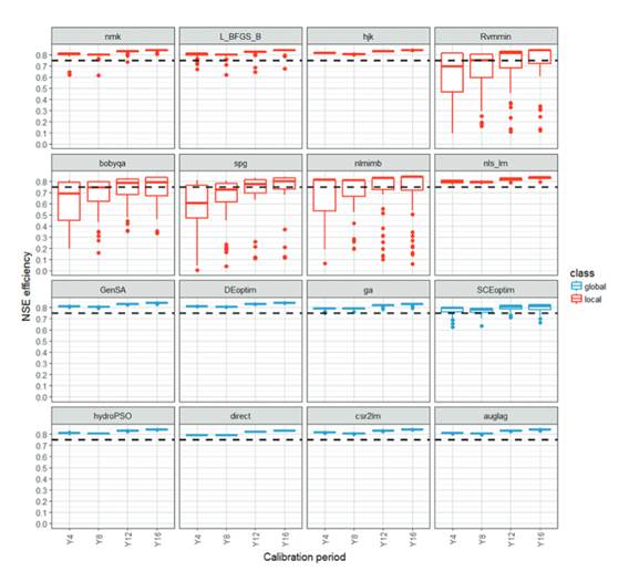
Figure 2 Performance of optimization methods in terms of NSE efficiency for various calibration periods. Black dash line is set at satisfactory level (NSE = 0.75). 

Regardless of the duration of the calibration period, global methods generally outperform local methods. Local methods Rvmmin, bobyqa, spg and nlmimb, which exhibit the lowest model performance of the entire group, are an example of this. Even when these four methods were able to find high NSE values, above the satisfactory threshold of 0.80, their NSE distributions are much more dispersed and therefore less reliable. Local methods are in general; more sensitive to getting trapped in local minima from where they are unable to escape, particularly if different sets of initial model parameters are considered. Furthermore, the presence of numerous outliers suggests that this is most likely to be the consequence of extreme sets of initial model parameters that ultimately lead to unstable solutions. In consequence, these four methods fail to achieve satisfactory optimal parameter sets. The remaining local methods, predominantly nls_lm and hjk are considerably more stable and more effective than the four methods abovementioned, as all their pairs are above NSE = 0.75. Local methods nmk and L-BFGS-B, even when showing a better performance than methods Rvmmin, bobyqa, spg and nlmimb exhibit, do exhibit some outliers, which suggest that these two methods are more prone to getting trapped in local minima as compared to nls_lm and hjk. For instance, nls_lm and hjk are considered the most reliable of the local methods. Global methods on the other hand, show a remarkably comparable NSE distribution, with stable median values, short inter-quartile ranges and rare or non-existent outliers, which translates into low sensitivity (variance) to initial model parameter values and higher reliability. This suggests that the HBV-TEC model parameter space has a definite, converging global structure which cannot be fully described by some local methods. SCEoptim however, seems to be an exception, since it shows wider distributions, lower median values, and higher numbers of outliers when compared to the other global methods, which indicates that SCEoptim is the most sensitive global method to initial sets of model parameters. This suggests that in most cases, SCEoptim is incapable of finding a distinguishable region of the global minima irrespectively of the calibration period. SCEoptim shows overlapping boxplots of similar proportions along with several outliers. This reduces reliability on SCEoptim and its capacity to properly identify HBV-TEC model parameters when compared to the remaining global methods. Contrastingly, local methods nls_lm and hjk show performances as good as or even better than SCEoptim.Since an optimization method should minimize the selected objective function as much as possible and exhibit a low sensitivity (variance) to initial model parameter values, the median and variance values of the NSE efficiency were used to create a normalized-metric ranking system that allowed for a simple and easy comparison of all optimization methods. The normalized-metric measures the performance of an optimization method in a scale varying from 0.0 to 1.0, with assigned relative weights of 0.5 for both the median and variance. Afterward, an absolute ranking varying from 0 to 16 was associated to each optimization method. For the sake of simplicity, this normalized metric was aggregated across all calibration periods.Consistently, global methods are ranked higher than local methods except for hjk and nls_lm, which perform better than SCEoptim (figure 3). Unvaryingly, Rvmmin, bobyqa, spg and nlmimb occupy the lowest rankings; supporting the notion that these are the least effective methods of them all. On the contrary, csr2lm, DEoptim and GenSA occupy the first three positions of the ranking, closely followed by hjk, which indicates that these are the most effective optimization methods. In an attempt to group the temporal-aggregated performance of all optimization methods, a Principal Components Analysis (PCA) was executed to transform the original variables into new variables that are independent and orthogonal (figure 4). PCA is a linear transformation technique that provides a smaller set of uncorrelated variables (called components) from a set of correlated variables while maintaining most of the information in the original data set (33). Clusters of homogeneous variables can then be highlighted, isolated and analyzed. The standardization to the same variance-scale avoids some variables becoming dominant due to differences in measurements, magnitudes and units.

PCA results shows that most of the total variance (58.9% + 22.2% = 81.1%) was captured in the first two principal components (figure 4a). Essentially, three independent clusters are clearly formed based on their unit-variance contribution and correlation. Cluster-1 includes Rvmmin, bobyqa, spg and nlmimb, which are the least effective methods. Cluster-2 includes all remaining methods (local and global) except L_BFGS_B which seems to behave independently, forming a third cluster (Cluster-3) by itself. Also, nls_lm exhibits a tendency towards independence but is still strongly related to Cluster-2. Optimization methods grouped within Cluster-2, which includes all global methods, show a strong positive correlation and are properly represented in terms of unit-variance, as their individual vectors (arrow lines) lay on top of one another and their magnitude reaches the outer circle, which represents the scaled unit-variance. Nevertheless, it can be seen that methods SCEoptim and nmk, even when strongly correlated to the remaining methods within Cluster-2, show a higher unit-variance since their individual vectors are closer to the origin than to the outer circle. This tendency is also consistent with the distribution (and therefore geometric similarities) of their respective boxplots (figure 2) and the normalized-metric ranking (figure 3).

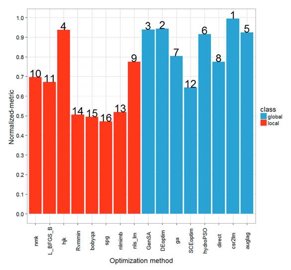
Figure 3 Normalized-metric and absolute ranking positions for the performance of various optimization methods 

This supports findings by Piotrowski et al. (⁹), who states that with a few exceptions, almost all global optimization methods perform similarly in terms of performance. Cluster-1 and Cluster-2 however, are uncorrelated since there is an angle of nearly 90 degrees between their grouped vectors. Cluster-1 has a strong representation in terms of unit-variance but is moderately represented in terms of correlation since its unit vectors are more dispersed as compared to Cluster-2. Cluster-3, only represented by L_BFGS_B, lies somewhere in between clusters 1 and 2. In essence, the NSE performance of the various optimization methods can be grouped in two main independent clusters, with method L_BFGS_B somewhere in between (figure 4b).

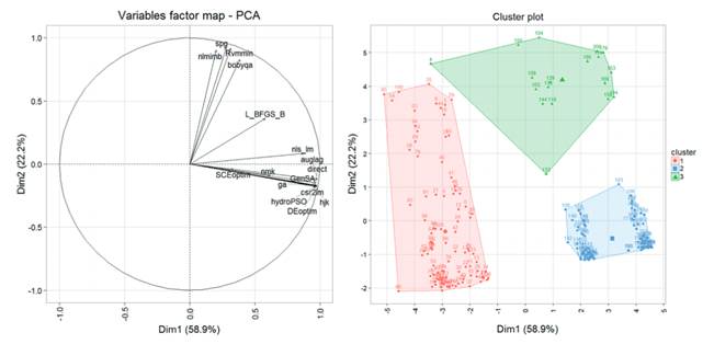
Figure 4. Calibration-period aggregated Principal Components Analysis (a) and cluster plot (b) of NSE efficiency for various optimization methods. 

Duration of the calibration period

Local methods Rvmmin, bobyqa, spg and nlmimb show a visible increase on NSE efficiency as the duration of the calibration period increases (figure 2), indicating that these methods are considerably sensitive to the duration of the calibration period. It seems that longer calibration series carry more information than shorter series and therefore reduce the tendency of these methods to become stuck at local minima. However, the remaining local and all global methods are less subject to this time-dependent performance, since the increase in NSE scarcely reaches 0.04 from Y4 to Y16 in most cases. Experimental results also show that longer calibration periods promote better model performance and possibly higher parameter identifiability. Conversely, if only short observation periods are available (in the order of 4 to 8 years) they still could be used in optimization with sufficient confidence. This is of course only valid for the upper Toro river catchment.

Computational cost

Scatter plots showing the performance of optimization methods in terms of NSE efficiency versus cost function calls for all 50 sets of initial model parameters are presented for each optimization method (figure 3). As abovementioned, each optimization method was executed using its default parameters and the maximum number of function evaluations allowed was set to 20000. Starting with local methods Rvmmin, bobyqa, spg and nlmimb, the choice of initial model parameter values heavily affects the capacity of these methods to find a feasible optimum solution.

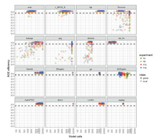
Figure 5 Performance of optimization methods in terms of NSE efficiency versus cost function calls for various optimization methods. Black dash line is set at satisfactory level (NSE = 0.75) 

An extremely dispersed behavior through the entire model domain, underlines that these methods are highly sensitive to get trapped in local minima in just a few calls. Methods Rvmmin and bobyqa can be stuck in local minima in as few as 200 model calls, exhibiting NSE values as low as 0.30 or below. On the other hand, method spg is both highly expensive and highly unreliable, as its computational cost reaches around 15000 calls and present a variation of NSE as low as 0 and as high as 0.84. Method L_BFGS_B, once again performed independently from all methods. Additionally, L_BFGS_B requires between 1000 and 20000 model calls, which represents a variation of three orders of magnitude, making this method as expensive as most global methods. As for the other local methods, hjk requires between 3000 and 20000 model calls to achieve NSE values over 0.80, basically, a fluctuation of one order of magnitude. Method nmk requires between 1000 and 5000 model calls. The situation is dramatically different nonetheless for nls_lm, as it is able to minimize the cost function in a range varying from 100 to 500 model calls. This is a significant difference of nearly two orders of magnitude as compared to hjk, nmk or L_BFGS_B but with comparable efficiencies. On the other hand, most global methods have similar computational costs when compared to the most effective local methods (hjk and nmk) except nls_lm, but show higher NSE independence and far less dispersion in general. Methods GenSA, HydroPSO and csr2lm exhibit very similar ranges of between 5000 and 20000 model calls, which make them very similar in terms of computational cost and NSE efficiency. Methods DEoptim, ga, direct and auglag, which only consider the upper and lower parameter bounds of the cost function and do not accept initial parameter values, show very little deviation in terms of model calls, since their ranges stay quite close to 18000, 8000, 20000 and 2000 model calls correspondingly. In consequence, these methods are able to locate a comparable region for the global minima regardless of the initial set of model parameters. Little or no distinction can be made among the various calibration periods (Y4 to Y16), suggesting that in most cases, the computational cost is independent from the calibration period. The only exception is SCEoptim, which seems to require fewer model calls as the duration of the calibration period increases (between 700 and 7500). Nonetheless, SCEoptim is unreliable as it presents higher NSE dispersions when compared to the other global methods. The only two methods that stand out in terms of computational cost are auglag (global) and nls_lm (local). If computational resources were limited, nls_lm could provide a good local minimum in around 500 model calls, whereas auglag could do it in around 2000 calls. Derived optimum parameters sets from these methods could then be used to run a more extensive global search using methods such as DEoptim, GenSA or csr2lm.In essence, the most effective local methods (except nls_lm) are as expensive as most global methods. Somehow, this discourages the use of local methods and promotes the use of global methods. Nonetheless, the effect of a lower-allowed maximum number of function evaluations (e.g. 10000, 5000 and 2000) for global methods should be studied, particularly for general operational purposes.

Conclusions and remarks

Eight global and eight local optimization methods were used to calibrate the HBV-TEC hydrological model. The following conclusions can be drawn:

The results of this study represent valuable instruments for the operational water management of the upper Toro river catchment, including river and flood forecasting, potential reservoir operation downstream and climate change modelling. However, even when these findings are solid, one catchment is not enough to draw general conclusions.

Acknowledgements

This research was supported by Vicerrectoría de Investigación at Instituto Tecnológico de Costa Rica (TEC). The author is grateful to Area de Hidrología, Centro de Servicio Estudios Básicos de Ingeniería & Construcción at Instituto Costarricense de Electricidad (ICE) for providing observed data for the Upper Toro River catchment.