I. Introduction

Hydrological studies require analyses of large amounts of hydrometeorological information related to precipitation, flows, temperature, and evaporation, among others.

The data collected represent raw information, but if properly organized and analyzed, they provide hydrologists with a very useful tool which allows them to make decisions in the design of hydraulic structures [⁵].

To make the calculations, hydrologists have to confront a series of problems:

Due to the complexity of information processing and of the calculations, errors can occur, making it useful to have software that provide hydrologists with a tool that enables them to simplify all these processes, and even to simulate their results, allowing them to optimize their design.

Objective

Create software which will facilitate and simplify complex calculations, and the analysis of the abundant information required in hydrological studies.

II. Theoretical basis

Random variables

A random variable [¹], is a function X, defined on a sample space S, which assigns a value to the variable for each point (or each result) of the sample space of an experiment.

Random variables are also known as stochastic variables whose values are real numbers which cannot be predicted with certainty before the phenomenon occurs; i.e., they occur randomly.

Discreet random variable

A random variable X is discrete when its values are restricted to a finite or infinite enumerable set.

Example: number of rainy days that occurred during the months of any year.

Continuous random variable

A random variable X is continuous when its values are within a continuous range, and may be represented by any whole or decimal number.

Example: the daily flow registered in a measuring station.

Distributions

The behavior of a random variable is described through its probability law, which may in turn be described in several ways. The most common is through the distribution of probabilities of the random variable [⁴].

Notation:

Distribution measurements

Arithmetic mean

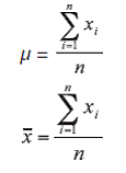
Given the composite sample of n data x ₁, x ₂, ..., x _n, the mean is defined as their algebraic sum, divided by the number of data. When the average is calculated for a population, it is denotedby µ, and when defined for a sample, it is denoted by x.

Mathematically speaking, the average of data that are not grouped is represented by:

where:

m = population mean

x = sample mean

xi = i^th value of the mean

xii n = number of data of the sample or population

The median

The median is a single value of a set of data which measures the central element in the data [⁵]. This single element of the data is the closest to the middle, or the most central value of a set of numbers. Half of the elements are above this point, and the other half are below it.

If x ₁ , x ₂ , x ₃ , ..., x _n are data organized in increasing or decreasing order, and n is an odd number, the median (Med) is the datum at the center, i.e.:

Med =, for an odd number n

if n is an even number, the median is the average of the central numbers, i.e.:

, for an even number n

The mode

Is the value that occurs most frequently in a set of data, denoted by Mo.

For data grouped in class intervals, once the modal class is defined, the mode is calculated using the following equation:

where:

Mo = mode

Lm = lower limit of the modal class

d1= difference between the frequency of the modal and pre-modal class (the class before the modal class)

d2= difference between the frequency of the modal and post-modal class (the class after the modal class)

w = range of the class interval

In general, the modal class is that which has the maximum frequency.

Variance

The variance of the population (σ²), is defined as the sum of squares of the deviations of the data with respect to the mean, divided by the total number of data, i.e.,:

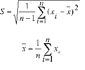
The variance of the sample (S²) [⁵], is obtained by dividing the sum of squares of observations of the data with respect to the mean by the total number of observations minus one, i.e.:

Standard deviation

The standard deviation is defined as the positive square root of the variance, i.e.:

(for the population)

(for the sample)

Coefficient of variation

This is a relative measurement of dispersion, which is related to the standard deviation and the mean, i.e.:

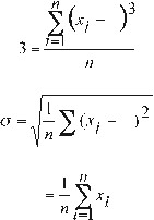
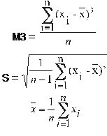
Bias

The bias is the statistics that measures symmetry and asymmetry [²].

The bias (γ) for data from the population is obtained with the following equation:

where:

The bias of data in the sample is obtained with:

Cs =

where:

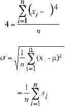
Kurtosis

For data of the population the kurtosis coefficient (k), is defined by the following equation:

where:

The kurtosis coefficient for data in the sample [²], is defined as:

where:

Estimation of parameters

The parameters of a theoretical distribution are variables that have a defined value for each set of data. Once the parameters are defined, the theoretical distribution is also defined.

In general, a density function or a cumulative distribution function may be expressed as a function of the random variable, and in general as a function of its parameters. For instance, the density function of the normal distribution of random variable X, is:

where:

µ = location parameter

σ²= scale parameter

To define the function f(x), the parameters µ and σ² must be calculated.

Since all the values of the random variable are usually unknown, the estimation of the parameters is made based on a sample [⁴].

Methods for the estimation of parameters

To determine the numeric values of the theoretical distribution parameters based on data in the sample, several estimation methods are used [⁵]; in order of ascending efficiency, they are:

Goodness-of-fit tests

The goodness-of-fit tests consist in verifying, graphically and statistically, if the empirical frequency of the series analyzed fits a previously selected theoretical probability function with parameters estimated based on values of the sample.

The purpose of statistical tests [⁴], is to measure the certainty obtained when a statistical hypothesis is made for a population, i.e., to evaluate the assumption that a random variable will be distributed according to a certain probability function.

The most used goodness-of-fit tests are:

Theoretical distributions

Hydrologists usually have a record of hydro-meteorological data available (precipitation, flows, evapotranspiration, temperatures, etc.). Based on their knowledge of the physical problem, they will choose a probabilistic model to use which will satisfactorily represent the behavior of a variable.

Normal or Gaussian distribution

A random variable X, is said to have a normal distribution [²], if its density function is:

or

for -∞< x <∞

where:

f(x) = normal density function of variable x x = independent variable

X = location parameter, equal to the arithmetic mean of x

S = scale parameter, equal to the standard deviation of x

EXP = exponential function with base e (napierian logarithms).

When the random variable X, is normally distributed with mean σ = X and variance (σ2 = S2), it is denoted as:

X ~ N ( X , S2)

Parameter log-normal distribution

The random variable X, is positive and the lower limit xo does not appear.

The random variable: Y = lnX, is normally distributed with mean γ y and variance σ2y.

These parameters are used to specify that the distribution is logarithmic, given that the mean and variance of X may also be used.

It is said that a random variable X, has a 2-parameter log-normal distribution [⁵], if its density function is:

for 0 < x <∞

Where µy, σy, are the media and the standard deviation of the natural logarithms of x, i.e., of lnx, and represent respectively the scale and the shape parameters of the distribution.

Parameter gamma distribution

It is said that a random variable X, has a 2-parameter gamma distribution [⁵], if its probability density function is:

for:

0 ≤ x <∞ 0 <γ<∞

0 < ß <∞

Where:

γ= shape parameter (+) ß = scale parameter (+)

Γ(γ) = complete gamma function, defined as:

which converges if γ> 0

Log-Pearson type III distribution

It is said that a random variable X, has a log-Pearson type II [⁵] distribution if its probability density function is:

for: xo ≤ x <∞

-∞< x_o<∞

0 < ß <∞

0 <γ<∞ where:

x _o = position parameter ß = scale parameter

γ = shape parameter

Gumbel distribution

The Gumbel distribution [⁵], is one of the extreme value distributions, also known as the Extreme Value Type I, Type I Fisher-Tippett or double exponential distribution.

The cumulative distribution function of the Gumbel distribution, has the form: F(x) = EXP(-EXP(-(x - µ) /α)) or

for: -∞< x <∞

where:

0 <α<∞, is the scale parameter

-∞< µ <∞, is the position parameter, also called the central value or mode

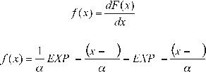
Deriving the cumulative distribution function with respect to x, the density function of probability is obtained, i.e.:

or

for: -∞< x <∞

Log-Gumbel distribution

The cumulative distribution function of the Gumbel distribution [⁵], has the form:

for: -∞< x <∞ where:

0 <α<∞, is the scale parameter

- ∞< µ <∞, is the position parameter, also called the central value or mode

If the variable x is replaced by lnx in the equation the cumulative function of the log-Gumbel distribution, or Fréchet distribution, is obtained.

Hydrometry is the branch of Hydrology that studies runoff measurement. Another term commonly used for the same purpose is flow measurement. To estimate a flow is to determine by measurement the flow that passes by a given section at a given moment [⁶].

Maximum flows To design [⁶]:

The design flow must be calculated or estimated, which in these cases are the maximum flows.

Some methods to calculate the maximum flow are:

Evapotranspiration

These are the total losses: evaporation from the evaporating surface (soil and water) + plant transpiration.

The term potential evapotranspiration [⁶] was introduced by Thornthwaite, and is defined as the total loss of water that would occur if there was never a lack of water in the soil to be used by vegetation.

Consumptive use is defined as the sum of evapotranspiration and water directly used to build plant tissue.

Since the amount of water used to build tissues is insignificant compared to that consumed in evapotranspiration, it may be said that:

Consumptive use » evapotranspiration

In irrigation projects, it is important to make initial calculations of the water required by crops. These water needs, which will be met through irrigation, are the evapotranspiration or consumptive use.

Methods based on meteorological data are used to calculate these amounts of water, of which the most well known are the Thornthwaite and Blaney -Clidde methods.

Materials and methods

Visual Basic, version 6.0 was used to develop the software, which permits the creation of 32-bit applications.

Numerical methods are be used to solve the equations, such as:

To calculate theoretical cumulative distributions such as the Normal, Log-Normal, and Gamma, and as to estimate their inverse values, series development is used.

Many solutions of the equations are found using nomograms and tables. In the process of computation, they should be transformed into equations; the following will be used to determine the most appropriate equations:

Results

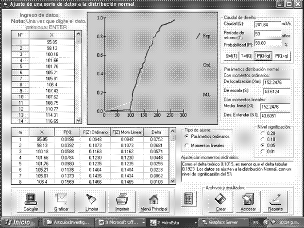
The product of this work is HidroEsta. The following figure shows one of its screens, with the calculation of the normal distribution:

Discussion

The results calculated using the application are in all cases more approximate than those obtained with nomograms.

HidroEsta represents a contribution to the simplification of hydrological studies. It is important because: