


 Inglês (pdf)
 Artigo em XML
 Referências do artigo
 Enviar este artigo por email
 Citado por SciELO
  Similares em
SciELO
Similares em
SciELO  uBio
uBio 
 Permalink
Introduction
Over the past few years, science of taxonomy has been suffering from dwindling number of experts (Rodman & Cody, 2003). Moreover, the pace of traditional taxonomy is also very slow. However, in the recent past, the pace of data gathering and analysis in taxonomy has been greatly increased by the development of information technology (Chen, Bart, & Teng, 2005). A family of software tools have been designed for gathering and analyzing data on morphometric variation from images of specimens (Rohlf & Bookstein, 1990). C. mrigala (Hamilton, 1822), (Cypriniformes: Cyprinidae) is a warm-water teleost, inhabitant of Indo-Gangetic riverine system spread across northern and central India, and the rivers of Pakistan, Bangladesh, Nepal and Myanmar (Reddy, 1999; Dahanukar, 2010). It has been effectively transplanted out of its natural range within India and parts of Asia as well as Europe (Chondar, 1999; Talwar & Jhingran, 1991). The major source of seed in India is contributed from natural resources. However, over the last few decades, wild capture fishery appears to be declined (Payne, Sinha, Singh, & Haq, 2004; FAO, 2006-2014) and changes in its distribution, phenotypic traits and biological characteristics have also been reported (Rao, 2001; Sharma, 2003). Therefore, it is essential to examine the stock structure of C. mrigala to overcome this fall in catch of this important Indian major carp.
The long-term isolation of populations and interbreeding can lead to morphometric variations between populations which can provide a basis for discriminating stocks (AnvariFar et al., 2011; Sajina, Chakraborty, Jaiswar, Pazhayamadam, & Sudheesan, 2011). There are many well-documented studies on population differentiation based on traditional morphometric characters (Turan, Yalcin, Turan, Okur, & Akyurt, 2005; Quilang, Basiao, Pagulayan, Roderos, & Barrios, 2007; Saini, Dua, & Mohindra, 2008). Now-a-days Studies of morphometric measurements based on truss network system (Strauss & Bookstein, 1982) constructed with the help of landmark points has been increasingly used for stock identification (Turan, Erg, Grlek, Bapusta, & Turan, 2004; Gopikrishna, 2006; Hossain, Nahiduzzaman, Saha, Khanam, & Alam, 2010; Ujjania & Kohli, 2011; Sajina et al., 2011; AnvariFar et al., 2011; Mir, Sarkar, Dwivedi, Gusain, & Jena, 2013; Sarkar, Mir, Dwivedi, Pal, & Jena, 2014).
Several studies have been conducted on the biology of Indian major carps viz. Labeo rohita, C. mrigala and C. catla, to study differentiation among the populations recently (Mir et al., 2012; Mir et al.,2013; Mir et al., 2014) and genetic variation (Zheng, Zheng, Zhu, Luo, & Xia, 1999; Chauhan et al., 2007; Luhariya et al., 2011; Luhariya et al., 2014; Das et al., 2012; Das et al., 2014; Hasant, Mollah, & Alam, 2015), however information available on morphometric variation in natural populations of these major carp is very limited and restricted to a particular region (Mir et al., 2013; Sarkar et al., 2014; Das et al., 2014). In the present communication, we therefore used multivariate statistical techniques to evaluate natural population structure on the size-free landmark based morphological variations of C. mrigala from major rivers of Ganga River basin. It is also necessary to mention here that some populations of the present study were included in the previous study on genetic variation of this economically important species (Chauhan et al., 2007). So, the results obtained from the present study will also be useful in correlation between genetic variation and morphological variation (Poulet, Berrebi, Crivelli, Lek, & Argillier, 2004).
Materials and methods
Study site: The river Ganga has it origin at the confluence of the Bhagirathi and Alaknanda, which descend from the upper Himalayas to Devprayag at an elevation of 4 100 m above mean sea level from the Gaumukh glacier in Uttarakhand, India. It flows south and east for some 2 525 km before reaching Bay of Bengal. The northern tributaries included in the present study are Sharda and Ghaghra and the southern tributaries include Chambal, Sindh, Kalisindh, Son and Tons. The River Banas originates in the Khamnor Hills of the Aravalli Range, about 5 km from Kumbhalgarh in Rajsamand district with approximately 512 km in length, is a tributary of Chambal, which in turn flows into the Yamuna. It flows northeast through the Mewar region of Rajasthan, and meets the Chambal near the village of Rameshwar in Sawai Madhopur District. Hiran River rises in the Bhanrer range in the Jabalpur district of Madhya Pradesh near the Kundam village at an elevation of 600 m and flows in a generally South-westerly direction for a total length of 188 km to join the Narmada from the right near Sankal village.
Sampling: A total of 381 specimens of C. mrigala were collected from ten different drainages of the Ganga River basin including main channel. The sample size and relative information for all the sampling sites selected to document morphometric variation are presented in table 1 and figure 1 (Table 1, Fig. 1).
Digitization of samples
Fish were placed on laminated graph sheets, body posture and fins were teased into a natural position. Each individual was labelled with a specific code for identification. A Cyber shot DSC-W300 digital camera (Sony, Japan) was used to capture the digital images. After image capture, each fish was dissected for sex determination by macroscopic examination of the gonads. The gender was used as the class variable in ANOVA to test for significant differences in morphometric characters, if any, between male and female.
Data collection: Two-dimensional Cartesian coordinates of 12 landmarks were recorded on the left view of each specimen (Fig. 2). Data were generated from digitalized images using a combination of three different softwares: tpsUtil was used for converting graphics images in to ‘tps’ format; tpsdig was used for fixing landmarks on the images and also setting scale for the image; PAST was used for generating truss data based on the landmarks (Rohlf, 2006). A total of 66 inter-landmark morphometric characters were extracted according to Strauss & Bookstein (1982).
Statistical analysis: The data generated by PAST were log-transformed (Strauss, 1985). Data was transformed in independent form to follow the Elliott, Haskard, & Koslow (1995): Madj = M(Ls/L0)b, where M is the original measurement, Madj the size adjusted measurement, L0 the standard length of the fish, Ls the overall mean of standard length for all fish from all samples in each analysis, and b estimated for each character from the observed data as the slope of the regression of log M on log L0using all fish from each group. Standard length (SL, character code 1-6) was excluded from the final analysis because SL was used as a basis for transformation (Mamuris, Apostolidis, Panagiotaki, Theodorou, & Triantaphyllidis, 1998) and thus 65 morphometric variables were retained.
Univariate analysis of variance (ANOVA) was performed for 65 morphometric characters to evaluate the significant difference among the three locations and those morphometric characters which showed highly significant variations (P < 0.01) were used to achieve the recommended ratio of the number of organisms measured (N) to the parameters included (P), in order to obtain a stable outcome from multivariate analysis (Johnson, 1981; Kocovsky, Adams, & Bronte, 2009).
The significant variables were subjected to linear discriminant function analyses (DFA) and principal component analysis (PCA) to discriminate the three populations. Principal component analysis helps in reduction of morphometric data (Veasey, Schammass, Vencovsky, Martins, & Bandel, 2001), in decreasing redundancy among the variables (Samaee, Mojazi-Amiri, & Hosseini-Mazinani, 2006) and in extracting a number of independent variables for population differentiation (Samaee, Patzner, & Mansour, 2009). In PCA, Jolliffe’s rule with eigen values of at least 0.7 was applied to retain principal components (Dunteman, 1989) and factor loading greater than 0.30 is considered significant, 0.40 more important and 0.50 or greater very significant (Nimalathasan, 2009). The Wilks’ k was used to compare the differences between and among all groups. The DFA was used to calculate the percentage of correctly classified (PCC). A cross-validation using PCC was done to estimate the expected actual error rates of the classification functions. Box plot was prepared for each discriminant morphometric characters. Statistical analyses for morphometric data were performed using the SPSS version 12 software package and Excel (Microsoft Office 2007).
Results
No significant difference was found in any of the morphometric characters between both sexes and therefore the data for both sexes were pooled for further analyses. No significant correlation was observed between any of the transformed morphometric variables and SL (P > 0.001), indicating that the effect of size was successfully removed. The analysis of variance (ANOVA) showed that fish samples from 10 locations differed significantly (P < 0.05) in all the65 transformed morphometric characters studied. In this study, the N:P ratio was5.86.
Principal component analysis using varimax rotation of 65 significant variables extracted eight principal components accounting for 94.1 % of the total variation (Table 2). Character code 1-3, 1-4, 1-5, 1-7, 1-8, 1-9, 2-4, 2-5, 2-6, 2-7, 2-8, 2-9, 3-4, 3-5, 3-6, 3-7, 3-8, 3-11, 4-9, 4-10,4-11, 4-12, 5-8, 5-9, 5-10, 5-11, 5-12, 6-8, 6-9, 6-10, 6-11, 6-12, 7-9, 7-10, 7-11, 7-12, 8-9, 8-10, 8-11, 8-12, 9-10, 9-11, and 9-12 showed significant on first principal component (PC1) which explained 68.6% variation of the total variation while character code 4-5, 4-6, 4-7, 5-8, 6-8 and 7-8 showed significant loading on PC2 which explained 6.8 % variation. Visual examination of plots of PC1 and PC2 scores revealed that specimens were grouped into 10 areas, with some degree of overlap among the populations (Fig. 3.).
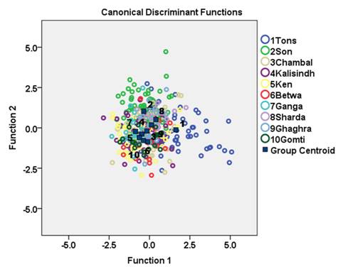
Forward stepwise discriminant function analysis of the 65 variables produced eight discriminating functions (DFs; Table 3). The first discriminant function (DF) accounted for 37.9 % while second DF accounted for 23.5 % of the among-group variability. The DF1 versus DF2 plot explained 61.4 % of total variance among the specimens and showed low distinction among C. mrigala stocks (Fig. 4.). Forward stepwise discriminant analysis of the all significant variables produced eight discriminating variables (Table 3). The morphometric measurements 10-11 and 2-6 showed highest variation on DF1, while 4-6 and 1-11 on DF2, 4-8 on DF3, 3-10 on DF5, 1-10 on DF6 and 8-9 contributed to DF8 (Table 3). The linear discriminant analysis gave an average PCC of 45.7 % for morphometric characters indicating low rate of correct classification of individuals into their original populations (Table 4).The percentage of correct classification ranged from 24.1 % to 65 %. It was highest for the stock of river Betwa (65 %) followed by river Gomti (63.2 %), Son (57.7 %), Tons and Ganga (50 %), Ken (44.7 %), Ghaghra (42.1 %), Sharda (40 %), Kalisindh (31.7 %) and lowest for river Chambal (24.1 %). The cross-validation test results were comparable to the results obtained from PCC (Table 4).
TABLE 1 Collection localities, sample size and size statistics (based on the Standard Length) of C. mrigala
| Rivers | Sampling sites | Coordinates | Sample size | Size range (cm) | Mean SL (cm) ± SD |
|---|---|---|---|---|---|
| Tons | Chakghat, Madhya Pradesh | 24o78'15'' N 81o78' 20'' E | 62 | 27.00-93.00 | 51.30±15.85 |
| Son | Beohari, Madhya Pradesh | 24o1' 20'' N 81o23'35'' E | 78 | 16.00-92.00 | 51.31±17.00 |
| Chambal | Kota, Rajasthan | 26o14' 38'' N 78o10'12'' E | 58 | 28.00-92.00 | 53.54±14.14 |
| Kalisindh | Shivpuri, Madhya Pradesh | 25° 26' 60'' N 77° 39' 0" E | 41 | 16.00-85.00 | 46.22±15.60 |
| Ken | Patan, Madhya Pradesh | 24o41' 40'' N 79o54' 95'' E | 38 | 16.00-92.00 | 51.38±17.60 |
| Betwa | Bhojpur, Madhya Pradesh | 23o45' 39'' N 78o14' 93' E | 20 | 30.50-80.00 | 47.08±125.36 |
| Ganga | Narora, Uttar Pradesh | 28°4'14" N 78°44'54" E | 26 | 31.00-71.00 | 47.69±10.76 |
| Sharda | Palia, Uttar Pradesh | 22° 49'60'' N 75° 47' 60'' E | 20 | 30.80-92.00 | 50.30±16.59 |
| Ghaghra | Faizabad, Uttar Pradesh | 26o75' 25" N 81o99'40'' E | 19 | 26.50-88.00 | 45.89±14.86 |
| Gomti | Lucknow, Uttar Pradesh | 26052'22" N 80054'58" E | 19 | 16.00-85.00 | 45.25±18.47 |
TABLE 2 Eigen values, percentage of variance and percentage of cumulative variance for the 8 PCs in case of morphometric measurements for C. mrigala
| Component | Initial Eigenvalues | ||
|---|---|---|---|
| Eigen-values | % of Variance | Cumulative % | |
| 1 | 44.590 | 68.599 | 68.599 |
| 2 | 4.414 | 6.791 | 75.391 |
| 3 | 4.061 | 6.247 | 81.638 |
| 4 | 2.778 | 4.274 | 85.911 |
| 5 | 1.651 | 2.539 | 88.451 |
| 6 | 1.398 | 2.150 | 90.601 |
| 7 | 1.210 | 1.861 | 92.462 |
| 8 | 1.047 | 1.611 | 94.073 |
TABLE 3 Contribution to discriminant functions (DFs) of morphometric variables of C. mrigala collected from 10 locations (*indicates largest absolute correlation between each variable and any discriminant function)
| Character code | DF1 (37.9%) | DF2 (23.5%) | DF3 (19.4%) | DF4 (6.9%) | DF5 (5.6%) | DF6 (3.8%) | DF7 (2,4%) | DF8 (0.5%) |
| 10-11 | -.842* | .260 | .329 | -.066 | .228 | .037 | -.194 | .143 |
| 2-6 | .566* | -.169 | -.520 | .213 | .006 | .254 | .509 | .107 |
| 4-6 | .176 | -.642* | -.011 | -.035 | -.353 | .163 | .074 | .632 |
| 1-11 | -.267 | .565* | .337 | -.224 | -.550 | .371 | -.071 | .020 |
| 4-8 | -.335 | -.048 | .665* | -.424 | .269 | -.202 | -.144 | .360 |
| 3-10 | .437 | -.105 | -.079 | .203 | .751* | .391 | -.128 | .133 |
| 1-10 | -.380 | .450 | -.243 | -.157 | -.179 | .630* | .327 | .182 |
| 8-9 | .305 | -.306 | .204 | .143 | .418 | .302 | .427 | -.550* |
TABLE 4 Percentage of specimens classified in each group and after cross validation for morphometric measurements for C. mrigala from ten drainages of Ganga River basin 45.7 % of original grouped cases correctly classified, 39.1 % of cross-validated grouped cases correctly classified
| Rivers | Tons | Son | Chambal | Kalisindh | Ken | Betwa | Ganga | Sharda | Ghaghra | Gomti | Total |
| Original (%) | |||||||||||
| Tons | 50.0 | 16.1 | 3.2 | 3.2 | .0 | 12.9 | 1.6 | 9.7 | .0 | 3.2 | 100.0 |
| Son | 1.3 | 57.7 | 2.6 | 3.8 | 6.4 | 2.6 | 5.1 | 7.7 | 6.4 | 6.4 | 100.0 |
| Chambal | 6.9 | 5.2 | 24.1 | 6.9 | 17.2 | 1.7 | 8.6 | 10.3 | 8.6 | 10.3 | 100.0 |
| Kalisindh | 9.8 | 2.4 | 9.8 | 31.7 | 12.2 | .0 | 19.5 | 2.4 | .0 | 12.2 | 100.0 |
| Ken | 10.5 | 2.6 | 7.9 | 10.5 | 44.7 | 2.6 | 15.8 | .0 | 2.6 | 2.6 | 100.0 |
| Betwa | .0 | .0 | 15.0 | .0 | .0 | 65.0 | 10.0 | 5.0 | .0 | 5.0 | 100.0 |
| Ganga | .0 | 11.5 | 3.8 | 19.2 | .0 | 7.7 | 50.0 | .0 | 7.7 | .0 | 100.0 |
| Sharda | 10.0 | 5.0 | 5.0 | 5.0 | 10.0 | .0 | 5.0 | 40.0 | 20.0 | .0 | 100.0 |
| Ghaghra | .0 | 10.5 | .0 | .0 | 21.1 | .0 | 10.5 | 15.8 | 42.1 | .0 | 100.0 |
| Gomti | .0 | .0 | 10.5 | 10.5 | 10.5 | 5.3 | .0 | .0 | .0 | 63.2 | 100.0 |
| Cross-validated (%) | |||||||||||
| Tons | 46.8 | 16.1 | 3.2 | 4.8 | .0 | 12.9 | 1.6 | 11.3 | .0 | 3.2 | 100.0 |
| Son | 2.6 | 52.6 | 2.6 | 5.1 | 6.4 | 2.6 | 5.1 | 7.7 | 7.7 | 7.7 | 100.0 |
| Chambal | 6.9 | 5.2 | 19.0 | 6.9 | 17.2 | 5.2 | 8.6 | 10.3 | 8.6 | 12.1 | 100.0 |
| Kalisindh | 9.8 | 2.4 | 9.8 | 26.8 | 14.6 | .0 | 22.0 | 2.4 | .0 | 12.2 | 100.0 |
| Ken | 10.5 | 2.6 | 5.3 | 13.2 | 42.1 | 2.6 | 15.8 | .0 | 5.3 | 2.6 | 100.0 |
| Betwa | .0 | .0 | 15.0 | .0 | .0 | 60.0 | 10.0 | 5.0 | .0 | 10.0 | 100.0 |
| Ganga | .0 | 15.4 | 3.8 | 19.2 | .0 | 7.7 | 46.2 | .0 | 7.7 | .0 | 100.0 |
| Sharda | 10.0 | 5.0 | 5.0 | 5.0 | 10.0 | .0 | 5.0 | 15.0 | 45.0 | .0 | 100.0 |
| Ghaghra | .0 | 10.5 | .0 | .0 | 21.1 | .0 | 10.5 | 42.1 | 15.8 | .0 | 100.0 |
| Gomti | .0 | .0 | 10.5 | 10.5 | 10.5 | 10.5 | .0 | .0 | .0 | 57.9 | 100.0 |
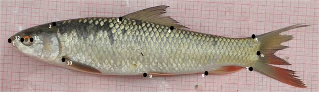
Fig. 2 Locations of 12 landmarks and truss network used for shape analysis. Land marks refer to 1. anterior tip of snout at upper jaw 2. most posterior aspect of neurocranium (beginning of scaled nape) 3. origin of dorsal fin 4. end of dorsal fin 5. anterior attachment of dorsal membrane from caudal fin 6. posterior end of vertebrae column 7. anterior attachment of ventral membrane from caudal fin 8. origin of anal fin 9. insertion of pelvic fin 10. insertion of pectoral fin 11. posterior end of eye 12. anterior end of eye.
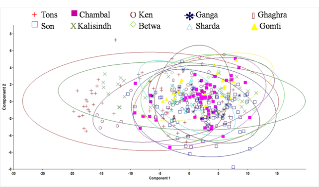
Fig. 3 Plot of the factor scores for PC1 and PC2 of morphometric measurements for C. mrigala from ten drainages of Ganga River basin.
Discussion
Information on stock structure of any species is very useful in developing conservation strategies for effective management of the natural fish populations. The present study deals with the distribution and pattern of morphometric variation in natural populations of C. mrigala estimated from truss network system. In fish morphology studies, inadequate sample size for multivariate analysis is a subject of question. In past, workers on PCA and DFA suggested that the ratio of the number of organisms (N) relative to the significant morphometric variables (P) in the study be at least 3-3.5 (Johnson, 1981; Kocovsky et al., 2009). Small N values may fail to adequately capture covariance or morphological variation, which may lead to false conclusions regarding differences among groups (McGarigal, Cushman, & Stafford, 2000). AnvariFar et al. (2011) found N:P ratio to be 4.32 in case of C. c. gracilis from Tajan River. However, Mir et al. (2013) reported N:P ratio to be 14.03 in L. rohita.
Discriminant function analysis (DFA) could be a useful method to distinguish different stocks of the same species (Karakousis, Triantaphyllidis, & Economidis, 1991). In the present study, low morphological differences between populations may be exclusively associated to body shape variation and not to size effects which were effectively removed by allometric transformation (AnvariFar et al., 2011). On the other hand, size-related characters play a predominant job in morphometric examination and the results may be flawed if not adjusted prior to statistical analyses of data (Tzeng, 2004). This segregation was partly confirmed by PCA, where the loadings of principal components revealed relatedness between populations. Common ancestry in the prehistoric period and possible exchange of individuals between rivers in different river basins could have been responsible for the observed low level of morphometric differentiation among wild mrigal populations. Das et al. (2014) also studied population structure of C. mrigala from peninsular riverine systems of India using truss landmark based morphometric analysis and indicated low morphometric differences among mrigal populations despite those populations from different geographic locations. Nautiyal & Lal (1988) also observed low morphometric differentiation among T. putitora populations in upstream of Ganga River. Similarly, several studies reported low morphometric differentiation in T. ilisha of Ganga and Hooghly River (Hora & Nair, 1940; Pillay, 1957; Sugunan & Das, 1996).
Primitive rivers like Indus, Ganga and Brahmaputra are formed during the late Pleistocene (Daniel, 2001) while Satluj, Beas, Yamuna, Ghagara and other Himalayan rivers were formed as lateral rivers to the Ganges more recently. Assuming that the fish stocks are distributed in space as gradients (Murta, Abaunza, & Cardador Sanchez, 2008), it is likely that fish from one tributary could belong to another, within the basin. The classification results of discriminant function clearly support this theory. The similarity between the stocks within a basin may be due to a common environment, similar genetic origin at earlier period, and the similarity may also be due to the genetic introgression of the fishes especially those in the transition zones. Study conducted by Hasant et al. (2015) on microsatellite DNA marker analysis revealed low genetic variation in the wild (three rivers namely the Halda, the Padma and the Jamuna) and captive (three hatcheries such as Brahmaputra, Raipur, and Sonali) populations of Cirrhinus cirrhosus. Luhariya et al. (2014; 2012) also reported low to moderate genetic divergence estimated from mtDNA cyto b and ATPase6/8 gene sequence in the natural populations of L. rohita among the major river systems of Indus and Ganges basins may result from gene flow across common flood plains. Das et al. (2014) also observed low genetic structure using mitochondrial DNA gene, cytochrome b among mrigal populations from peninsular riverine systems of India despite those populations from different geographic locations. Das et al. (2012) also reported low to moderate genetic diversity in wild Catla catla populations assessed through mtDNA cytochrome b sequences. Chauhan et al. (2007) also reported low genetic divergence estimated from allozyme and microsatellite markers in the natural populations of C. mrigala among the major river systems of Indus and Ganges basins may result from gene flow across common flood plains.
However, in the previous study on landmark based morphometry of Labeo rohita from six Indian rivers viz. Ganga, Ghaghra, Ken, Sharda Betwa, and Gomti of Ganga basin, Mir et al. (2013) reported significant variations among the populations. Sarkar et al. (2014) also reported high morphometric variation among the populations in C. catla collected from three rivres viz. Ken, Betwa and Ganga. Ujjania & Kohli (2011) also reported morphological difference in C. catla inhabiting MBS (large reservoir), SD (medium reservoir) and AP (small pond) in southern Rajasthan. In other major carps, Hossain et al. (2010) applied DFA and PCA on three populations of L. calbasu from Jamuna, Halda and Hatchery and reported high morphological discrimination among them due to the environmental factors and local migration of the fish.
The separation of the stocks within the basin may be due to different biotic and abiotic factors such as food availability, salinity, temperature, which are affecting the morphometry of a fish (Rohfritsch & Borsa, 2005). Morphometric variation of a fish can be subjective to genetic, environment and the interaction between both (Cadrin, 2000). Correlation between genetic variation and morphological variation has been confirmed in natural populations (Poulet et al., 2004) and both have been widely used in population differentiation (Buth & Crabtree, 1982; Agnese, Teugels, Galbusera, Guyomard, & Volckaert, 1997; Ibanez-Aguirre, Cabral-Solis, Gallardo-Cabello, & Espino-Barr, 2006; Das et al., 2014). The individual’s phenotype is more acquiescent to environmental influence is of particular importance during the early development stages (Pinheiro, Teixeira, Rego, Marques, & Cabral, 2005). The phenotypic variability may not necessarily reflect population differentiation at the molecular level (Ihssen et al., 1981). Apparently, the fragmentation of river impoundments can lead to an enhancement of pre-existing genetic differences, providing a high inter-population structuring (Esguicero & Arcifa, 2010).
In this study, the landmark protocol revealed low distinctness among the populations observed from different drainages of Ganga basin in India. Application of other stock identification tools such as life history properties, otolith chemistry, tagging experiments and genetic studies in coherent manner would be effective for planning proper management decisions and restoration of the natural populations of mrigal in the river ecosystem. The outcomes of this study would offer essential information to resource enhancement and help in delineating populations for fishery management of this commercially important fish species.

