


 Inglês (pdf)
 Artigo em XML
 Referências do artigo
 Enviar este artigo por email
 Citado por SciELO
  Similares em
SciELO
Similares em
SciELO  uBio
uBio 
 Permalink
One objective of roadkill surveys is the reduction of traffic accidents caused by collisions with wildlife, increasing safety for road users and preserving the biodiversity (Van der Ree, Smith, & Grilo, 2015). In the United States, material damage from collisions of this nature is estimated to exceed $ 1 billion and 1 500 people have died in such accidents over the past 10 years (Grilo, Bissonette, & Cramer, 2010). One million animals die each day from fatal accidents with vehicles in that same country (Forman, 1998). In this way, wildlife roadkill is one of the negative effects caused by roads that have been more widely studied (Forman & Alexander, 1998; Trombulak & Frissell, 2000; Coffin, 2007; Laurance, Goosem, & Laurance, 2009; Van der Ree et al., 2015).
In Brazil, the most conservative rate points to 14.7 (± 44.8) million animals being killed in a car accident every year (Dornas, Kindel, Bager, & Freitas, 2012), while another research indicates a rate as big as 475 million animals/year (Centro Brasileiro de Ecologia de Estradas, 2017). These data indicate the urgency of studies addressing this issue, in order to reduce the loss of biodiversity and public expenditures (Bager, Piedras, Martin, & Hóbus, 2007). Nevertheless, studies focusing on wildlife roadkill aggregation are recent in this country (Coelho, Kindel, & Coelho, 2008; Esperandio, 2011; Bueno, Freitas, Coutinho, Oswaldo Cruz, & Castro Júnior, 2012; Santana, 2012; Teixeira et al., 2013; Ferreira, Ribas, Casella, & Mendes, 2014; Carvalho, Iannini Custodio, & Marçal Junior, 2015; Ascensão, Desbiez, Medici, & Bager, 2017; Santos et al., 2017). Although it is not a focus of wildlife roadkill monitoring, domestic animals are also being killed on roads and because of their size, they can pose a threat to human safety. The studies that evaluate the domestic mammals’ roadkill hotspots (Esperandio, 2011) or that do at least a survey of the domestic fauna roadkill are rare (Bagatini, 2006; Freitas, 2009; Esperandio, 2011; Omena Junior, Pantoja-Lima, Santos, Ribeiro, & Aride, 2012).
It is essential to look for possible patterns of roadkill distribution, including domestic animals since these are responsible for a substantial amount of collisions (Esperandio, 2011). Roadkill aggregation zones, called hotspots, have been determined for several groups of wild animals, indicating that roadkill is usually not random (Clevenger, Chruszcz, & Gunson, 2003; Malo, Suárez, & Díez, 2004; Teixeira et al., 2013; Santos et al., 2017;) and hotspots can vary in time and space (Santos et al., 2017; Gonçalves et al., 2018). However, for domestic mammals the question still remains, is domestic mammals’ roadkill aggregated? Knowing where and when roadkill happens more frequently, enables one to identify critical points for the implementation of mitigation measures, such as fauna passages, fences, warning signs and electronic barriers (Glista, DeVault, & DeWoody, 2009; Grilo et al., 2010; Lesbarrères & Fahrig, 2012)
For domestic mammals, the occurrence of hotspots is probably different from those found for wild species, since the presence of domestic animals on the highways is due to very particular factors (Esperandio, 2011), human presence or abandonment being the most important. On the other hand, domestic and wild mammals’ roadkill could overlap because some domestic mammals act as scavengers and could be killed in the same sites as those of wild mammals (Slater, 2002; Schwartz, Williams, Chadwick, Thomas, & Perkins, 2018). Therefore, if hotspots of domestic animals overlap with those of wild species, they could be used to plan mitigation measures for a broad spectrum of species as proposed by Teixeira et al. (2013) for wild animals. In this context, the present study was undertaken to evaluate mammal roadkill aggregations in a Cerrado area, to locate these hotspots, to determine if wild and domestic mammal roadkill overlap and to explain through landscape analysis why these hotspots overlap or not.
Material and methods
Study Site: The survey was carried out on the stretch of the highway BR-050 between Uberlândia and Uberaba, Minas Gerais State, Brazil (Uberlândia, 18°54’46.19” S & 48°13’24.54” W; Uberaba, 19°43’59.29” S & 47°58’56.68” W) (Figure 1). The climate of the region presents seasonality, the rainy summer is from October to April and the dry winter from May to September (Rosa, Lima, & Assunção, 1991). The study area is in the Cerrado biome, which has campos, forest formations, gallery forest and veredas (Araújo & Haridasan, 1997). On the other hand, the intense agricultural activity reduced the Cerrado to small and isolated fragments (Araújo, Nunes, Rosa, & Resende, 1997). In this section of the BR-050, the highway crosses the rivers Uberaba and Uberabinha, some streams and several veredas or palm swamps. This highway is approximately 96 km and is a paved four-lane road. The road has hard shoulders and median strips. In April 2015, around 218 839 vehicles passed through the BR-050 highway (Concessionária de rodovias Minas Gerais Goiás S/A, 2018).
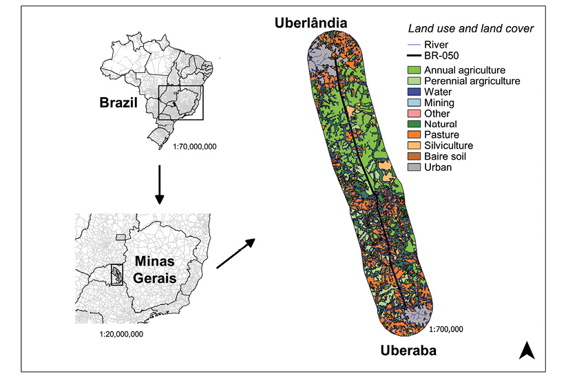
Figure 1 Study area highlighting land use and land cover in a 10 km buffer around the BR-050 highway, Uberlândia-Uberada, Minas Gerais state, Brazil (2012-2013).
Procedures: The road was monitored weekly, from April 2012 to March 2013, by car, at an average speed of 60 km/h, with two observers looking for roadkills on the highway. The monitoring trip started at 07:30 in the morning and lasted for the time necessary to cover the entire stretch. As the highway is a four-lane road, being the opposite lanes separated by a median strip, it was monitored in both directions (from Uberlândia to Uberaba, and from Uberaba to Uberlândia), totaling 192 km traveled weekly, 42 trips and 8 064 km at the end of one year of data collection, representing a sampling effort of 22.1 km/day.
After registration, we removed the carcass from the highway to avoid further recounts. Mammals’ roadkill identification was carried out based on Reis, Peracchi, Fragonezi, & Rossaneis (2010). We also consulted specialists to confirm these identifications. We only included in the analysis those animals whose identification allowed for grouping them safely in wild or domestic categories.
In order to get data from the landscape, we used a map of land use and land cover produced by the Ministry of the Environment, with a 1:250 000 scale and made based on satellite images from 2013 (Ministério do Meio Ambiente, 2015). We split the highway into 96 segments of 1 km each and created a buffer of this same size around each segment. Then, we quantified the area in this buffer for each one of these categories: agriculture, pasture, silviculture and natural cover. For each segment, we also calculated the distance to the nearest river (D_river), to the urban perimeter (D_urban) and to the nearest fragment of natural cover (D_fragment). Finally, we reckoned the number of fragments (N_fragments), the area of the smallest and largest natural fragment (S_fragment, L_fragment) and the presence of a river (River_presence) within the buffer area for each segment.
Data analyses: The 2D Ripley’s K-Statistics test from Siriema v1.1 software tests the existence or not of roadkill aggregations in different scales (Coelho, Coelho, Kindel, & Teixeira, 2011). The function L(r) used for the interpretation of the test results allows for evaluating the intensity of aggregation in different scales. An initial radius of 100 m, a radius increase of 500 m, a confidence level of 95 % and 1 000 simulations were used (modified from Coelho et al., 2011; Cáceres, Casella, & Goulart, 2012;Teixeira et al., 2013). The values of initial radius and radius increment corresponded to the scale at which mitigation measures could be effective (Teixeira et al., 2013).
We used the 2D HotSpot Identification test to identify where the roadkill aggregations were localized (Coelho et al., 2011). The Nevents - Nsimulated function used to interpret the test results allows to assess at what locations on the highway roadkill aggregations were located. We used a radius of 500 m because the lower the range of analysis, the more detailed the results are, scale in which the roadkill aggregations were significant, according to the results of the 2D Ripley K-Statistics test. A confidence level of 95 % and 1 000 simulations were used. Uberlândia city was the km zero and Uberaba city the km 96.
In order to compare if the roadkill hotspots’ location were similar between the different groups, we used the same procedure that Teixeira et al. (2013) used. The sections of the highway were considered sample units, the Siriema program calculates an aggregation index for each section of the highway (500 sections of 192 m each) (Coelho et al., 2011). We transformed the aggregation intensity data into binary variables representing the roadkill hotspots presence/absence (Teixeira et al., 2013; Santos et al., 2017). We corrected wild and domestic mammals aggregations position by ± 1 and 2 km. Than we performed a phi correlation in order to assess the similarity of wild and domestic mammals hotspots location using sjstats package (Lüdecke, 2018) in R 3.4.1 program (R Core Team, 2018).
In order to understand what kind and how land use influences roadkill hotspots, we created GLM models. First, we investigated multicollinearity among predictors using the Variance Inflation Factors (VIF) from the package car (John & Weisberg, 2011) (Table 1). We excluded variables Pasture and L_fragment that had a VIF > 10 (Montgomery & Peck, 1992) and that were less correlated to the response variables (Appendix 1 and Appendix 2). The response variable was the presence/absence of roadkill hotspot in each segment (we used a binomial distribution and a logit link function). We ran GLM analyses using GLmulti package in R (Calcagno, 2015) and set a maximum of four variables per model in order to facilitate models’ interpretation. Model selection was performed using the Akaike Information Criterion for small samples (AICc), retaining all models within ∆AICc < 2. We calculated AICc weights (wAICc) to compare the relative support of each model. The Area Under Cover (AUC) was calculated using epiDisplay package (Chongsuvivatwong, 2018). The Relative Importance Weight (RIW) was reckoned for the variables to understand the importance of each one using package GLmulti (Calcagno, 2015) (RIW > 0.9, strong effect; 0.9-0.6, moderate; 0.6-0.5, weak). We ran these tests in R 3.4.1 program (R Core Team, 2018).
Table 1: Variance Inflation Factors (VIF) for land use and land cover independent variables, BR-050 highway, Uberlândia-Uberaba, Minas Gerais state, Brazil (2012-2013)
| Variables | VIF - without exclusion | VIF - 1 exclusion | VIF - 2 exclusions |
| Agriculture | 21.84476 | 6.340877 | 4.047764 |
| D_fragment | 8.807212 | 8.466067 | 6.149074 |
| D_river | 2.855073 | 2.450321 | 4.238801 |
| D_urban | 3.338178 | 3.322098 | 2.706591 |
| L_fragment | 14.32365 | 12.90922 | excluded |
| N_fragments | 7.529584 | 7.269773 | 4.273296 |
| Natural | 23.52738 | 22.57528 | 4.644611 |
| Pasture | 14.91319 | excluded | excluded |
| River_presence | 1 | 1 | 1 |
| S_fragment | 2.732065 | 2.738433 | 3.020286 |
| Silviculture | 3.533716 | 1.859377 | 3.079449 |
In the second column, VIF was calculated for all land use and land cover independent variables. In the third column, VIF was calculated after excluding the variable Pasture (based on its relation to the answer variables in Appendix 1 and Appendix 2). In the fourth column, VIF was calculated after excluding the variables Pasture and L_fragment (the maintenance of the variable Natural instead of L_fragment was an ecological choice). We considered an acceptable VIF < 10 (Montgomery & Peck, 1992).
Results
We found 482 mammals’ roadkill, including 260 (54 %) wild mammals, 164 (34 %) domestic animals and 58 (12 %) were not possible to determine if they were wild specimens or not. Of the 21 recorded mammal species, five were domestic/exotic. The wild species most killed were: Cerdocyon thous, Euphractus sexcinctus and Conepatus semistriatus; the domestic ones were: Canis familiaris and Felis catus (Table 2).
Table 2: Mammals’ roadkill on BR-050 highway, Uberlândia-Uberaba, Minas Gerais state, Brazil (2012-2013)
| Taxa | N | C %¹ | Roadkill rate² |
| Mammalia (non identified species) | 43 | 8.9 | 0.53 |
| Didelphimorphia Didelphidae Didelphis albiventris Lund, 1840 | 7 | 1.5 | 0.08 |
| Lutreolina crassicaudata (Desmarest, 1804) | 2 | 0.4 | 0.02 |
| Pilosa Myrmecophagidae (non identified species) | 1 | 0.2 | 0.01 |
| Myrmecophaga tridactyla Linnaeus, 1758 | 3 | 0.6 | 0.03 |
| Tamandua tetradactyla (Linnaeus, 1758) | 14 | 2.9 | 0.17 |
| Cingulata Dasypodidae (non identified species) | 15 | 3.1 | 0.18 |
| Cabassous sp. McMurtie, 1831 | 3 | 0.6 | 0.03 |
| Dasypus novemcinctus Linnaeus, 1758 | 10 | 2.1 | 0.12 |
| Dasypus sp. Linnaeus, 1758 | 5 | 1.0 | 0.06 |
| Euphractus sexcinctus (Linnaeus, 1758) | 44 | 9.1 | 0.54 |
| Perissodactyla Equidae Equus caballus Linnaeus, 1758 * | 1 | 0.2 | 0.01 |
| Artiodactyla Suidae Sus domesticus Erxleben, 1777 * Primates | 1 | 0.2 | 0.01 |
| Cebidae Callithrix penicillata (É. Geoffroy, 1812) | 3 | 0.6 | 0.03 |
| Carnivora (non identified species) | 1 | 0.2 | 0.01 |
| Canidae (non identified species) | 10 | 2.1 | 0.12 |
| Canis familiaris Linnaeus, 1758 * | 100 | 20.7 | 1.24 |
| Cerdocyon thous (Linnaeus, 1758) | 52 | 10.4 | 0.64 |
| Chrysocyon brachyurus (Illiger, 1815) | 8 | 1.7 | 0.09 |
| Lycalopex vetulus (Lunda, 1842) | 8 | 1.7 | 0.09 |
| Felidae Felis catus Linnaeus, 1758 * | 61 | 12.7 | 0.75 |
| Leopardus pardalis (Linnaeus, 1758) | 1 | 0.2 | 0.01 |
| Leopardus sp. Gray, 1842 | 1 | 0.2 | 0.01 |
| Mephitidae Conepatus semistriatus (Boddaert, 1785) | 43 | 8.9 | 0.53 |
| Mustelidae Galictis cuja (Molina, 1782) | 4 | 0.8 | 0.04 |
| Procyonidae Procyon cancrivorus (Cuvier, 1798) | 20 | 4.1 | 0.24 |
| Lagomorpha Leporidae Lepus europaeus Pallas, 1778 * | 1 | 0.2 | 0.01 |
| Rodentia (non identified species) | 4 | 0.8 | 0.04 |
| Caviidae Hydrochoerus hydrochaeris (Linnaeus, 1766) | 13 | 2.7 | 0.16 |
| Erethizontidae Coendou prehensilis (Linnaeus, 1758) | 3 | 0.6 | 0.03 |
The wild mammals’ roadkill rate was 0.03 (± 0.02) individuals/km/day, with at least two animals per day, at most 17, and an average 6.26 (± 3.47) wild animals. The monthly roadkill rate was 0.98 (± 0.54) individuals/km/month. The annual roadkill rate was 11.90 (± 6.60) individuals/km/year. The domestic mammals’ roadkill rate was 0.02 (± 0.01) individuals/km/day, with at least one animal being found per day, at most 11 and an average 3.71 (± 2.20) domestic mammals. The monthly roadkill rate was 0.61 (± 0.33) individuals/km/month. The annual roadkill rate was 7.42 (± 4.17)individuals/km/ year.
Wild and domestic mammals showed roadkill aggregation (Figure 2). The roadkill aggregations of wild mammals were located at km: 15, 17, 20 to 23, 25, 47, 86, 90 to 91; with greater intensity at km 23 and 91 (Figure 3). The hotspots of domestic mammals were located at km: 2, 5 to 6, 37, 39 to 40, 44 to 45, 50 to 51, 69 to 71, 79, 93 to 95; with greater intensity at km 44 to 45, 50 to 51 and 70 (Figure 3). The roadkill hotspots of domestic mammals and wild mammals did not overlap (rphi = -0.06 P = 0.40), not even when we adjusted their location for one more km (rphi = 0.15, P < 0.001), neither for two (rphi = 0.24, P < 0.001) (Figure 4). From eleven wild mammal hotspots, just two (km 47 and 91) are within two km from a domestic mammal hotspot.
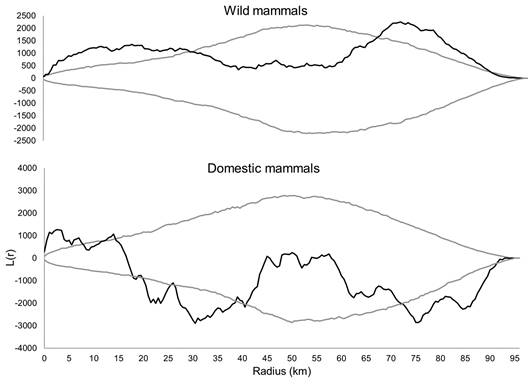
Figure 2 Radius at which there is roadkill aggregation for wild and domestic mammals on the BR-050 highway, Uberlândia-Uberaba, Minas Gerais state, Brazil (2012-2013). Results from the test 2D Ripley’s K-Statistics. Black line - L(r) function, gray lines - upper and lower confidence limits, when the black line is above the gray line it means that in that radius of analysis there are roadkill aggregations.

Figure 3 Location of wild and domestic mammals’ roadkill aggregations on BR-050 highway, Uberlândia-Uberada, Minas Gerais state, Brazil (2012-2013). Results from test 2D Hotspot Identification. Black line - The Nevents - Nsimulated funcion, gray lines - upper and lower confidence limits, when the black line is above the gray line it means that in that section of the highway there are roadkill aggregations.
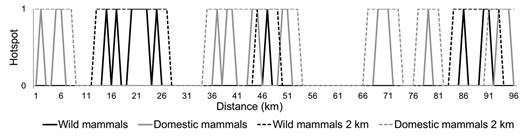
Figure 4 Comparison of the roadkill hotspots location for wild and domestic mammals on the BR-050 highway, Uberlândia- Uberada, Minas Gerais state, Brazil (2012-2013). We created a correction factor of ± two km around each hotspot for wild mammals (Wild mammals 2 km on the graph) and for domestic mammals (Domestic mammals 2 km on the graph).
Landscape models are excellent at explaining wild mammals’ hotspots, while for domestic mammals they are moderately good (Table 3). Wild mammals’ hotspots occur in larger agriculture and silviculture cover areas; near a river, a natural fragment and the urban perimeter (Table 4). Domestic mammals’ hotspots are localized near smaller silviculture areas, bigger natural fragments, far from a river and in more fragmented landscapes. The difference in the location of the wild and domestic mammals’ hotspots are associated with the effect of each variable, if the effect is negative for wild mammals, it is positive for domestic mammals and vice versa.
Table 3: Models that best explain hotspots location selected by AICc, BR-050 highway, Uberlândia-Uberaba, Minas Gerais state, Brazil
| Model | AICc | ∆AICc | weight | AUC |
| Wild mammals Null | 70.39 | 20.62 | ||
| + Agriculture + Silviculture - D_river - D_urban | 49.77 | 0.00 | 0.40 | 0.93 |
| + Agriculture + Silviculture - D_urban - D_fragment | 50.14 | 0.37 | 0.33 | 0.92 |
| Domestic mammals Null | 91.70 | 4.25 | ||
| - Silviculture + S_fragment + D_fragment | 87.45 | 0.00 | 0.05 | 0.75 |
| - Silviculture - River_presence + S_fragment | 88.38 | 0.93 | 0.03 | 0.73 |
| - Silviculture | 89.03 | 1.58 | 0.02 | 0.57 |
| - Silviculture + D_fragment | 89.11 | 1.66 | 0.02 | 0.65 |
| - Silviculture + S_fragment + N_fragments + D_fragment | 89.14 | 1.69 | 0.02 | 0.76 |
| - Silviculture - River_presence + S_fragment + D_fragment | 89.21 | 1.76 | 0.02 | 0.76 |
| - Silviculture - River_presence | 89.21 | 1.76 | 0.02 | 0.64 |
| - Silviculture + D_river + S_fragment | 89.23 | 1.78 | 0.02 | 0.72 |
AICc = Akaike Information Criterion for small samples; ∆AICc = difference between the AICc of a given model and that of the best model; AUC = Area under cover.
Table 4: Relative Importance Weight (RIW) and effect of the land use and land cover descriptor variables among all models, BR-050 highway, Uberlândia-Uberaba, Minas Gerais state, Brazil
| Wild mammals | Domestic mammals | |||
| Variables | RIW | Effect | RIW | Effect |
| Agriculture | 0.92 | + | 0.19 | - |
| D_fragment | 0.47 | - | 0.42 | + |
| D_river | 0.53 | - | 0.24 | + |
| D_urban | 0.87 | - | 0.19 | + |
| N_fragments | 0.04 | - | 0.23 | + |
| Natural | 0.10 | + | 0.21 | - |
| River_presence | 0.05 | + | 0.34 | - |
| S_fragment | 0.06 | - | 0.54 | + |
| Silviculture | 0.88 | + | 0.70 | - |
Discussion
The present study showed that nearly 30 % of the mammals’ roadkill included domestic animals. Omena Junior et al. (2012) found 16 % of domestic mammals among mammals’ roadkill, Freitas (2009) raised a total of 47 %, Esperandio (2011) recorded 28 % of domestic mammals and Bagatini (2006) 52 %. These authors also found Canis familiaris and Felis catus as the most killed domestic animals (Bagatini, 2006; Freitas, 2009; Esperandio, 2011; Omena Junior et al., 2012). Freitas & Barszcz (2015) analyzed news on the internet about wildlife vehicle accidents and concluded that 70 % involved domestic animals. All of these studies highlight the importance of domestic mammals’ roadkill, both because of their frequency, and because the group includes large animals, which leads to greater chances of serious accidents involving greater material and human losses.
Cerdocyon thous and Euphractus sexcinctus usually appears as the most killed species of wild mammals in Brazil (Dornas et al., 2012). Both species are common and adapted to living in disturbed environments, they are omnivorous and even eat dead animals on the road, the same being true for Conepatus semistriatus (Reis et al., 2010). The BR-050 highway presented a roadkill rate of 0.03 wild mammals/km/day which is relevant when compared to other researchers performed in a Cerrado region, 0.01 (Cunha, Moreira, & Silva, 2010; Carvalho, Bordignon, & Shapiro, 2014), 0.02 (Braz & França, 2016); 2.03 (Cáceres et al., 2012; Brum et al., 2018). Anyway, roadkill rates are underestimated and a correction index needs to be calculated in order to try to get more actual numbers (Santos, Carvalho, & Mira, 2011; Teixeira, Coelho, Esperandio, & Kindel, 2013).
The non overlapping of wild and domestic mammals’ hotspots can be explained by landscape characteristics since the effect of each environmental variable was different for wild and domestic mammal roadkill. Wild mammals’ roadkill hotspots were located near a river, other researchers concluded that the roadkill probability increases with proximity to a river (Bueno, Sousa, & Freitas, 2015; Ascensão et al., 2017). On the other hand, there are also results showing an opposite effect of this variable, as for Cerdocyon thous (Freitas, Oliveira, Ciocheti, Vieira, & Matos, 2015). Two different hypotheses can explain these results: 1) wild mammals have to move more when they are distant from rivers ending up being a roadkill victim; 2) wild mammals prefer to move close to a river increasing the roadkill probability near a river. Anyway, it seems that the response to river distance depends on the species. For domestic mammals, there were more roadkill hotspots far from rivers, probably because humans supply their necessity for water.
We found hotspots are near the urban perimeter, in these same sites a higher number of roadkill was observed for Myrmecophaga tridactyla (Ascensão et al., 2017) and Chrysocyon brachyurus (Freitas et al., 2015). This condition was the opposite of that observed for Dasypus novemcinctus and Tapirus terrestris (Ascensão et al., 2017). These results may indicate that species with a small home range will avoid urban areas and species with bigger home ranges overlap these areas increasing their probability of being killed inside an urban environment, however, this hypothesis needs investigation. Although from 17 domestic mammals’ hotspots, six are within 10 km from the urban areas, this variable is not important in explaining domestic mammals’ hotspots. Probably, other variables related to human presence will explain domestic mammal’s hotspots better, like the distance to the nearest farm or to a human building.
Wild mammal roadkill hotspots were associated with a higher cover of agriculture (Rezini, 2010; Santana, 2012) and silviculture. We can observe the contrary effect for domestic mammals. We believe that with the lack of natural areas, wild mammals have to use agriculture and silviculture areas to forage, reproduce and move. As these areas may have fewer food resources, they have to move more and consequently their chance of being killed is higher. Magioli et al. (2016) concluded that agricultural and fragmented landscapes still sustain high biodiversity and ecological functions. Lyra-Jorge, Ciocheti, & Pivello (2008) showed that silviculture areas maintain a similar biodiversity of medium and large-sized mammals when compared to natural Cerrado areas, executing an important function in connecting patches of native vegetation.
Wild mammals roadkill hotspots are near natural fragments. Bueno et al. (2015) report a positive relationship between the roadkill probability of large, arboreal and volant mammals and herbaceous vegetation cover. Ascensãoo et al., (2017) found that areas dominated by Cerrado had a higher roadkill probability for Cerdocyon thous and Euphractus sexcinctus. For domestic mammals, roadkill hotspots are located far from a natural fragment and when small fragments are bigger, since these animals are dependent on human care.
We conclude that wild and domestic mammals’ aggregations do not overlap, one factor that can explain this non overlapping is how landscape cover influences roadkill hotspot location with the effect of each variable being different between domestic and wild mammals. Models that explain wild mammals’ hotspots location are great, but domestic models are not, this might indicate that other factors that were not considered in this research may help explain domestic mammals’ hotspot location, as distance to the nearest farm, for example. On the other hand, this non overlapping can be a result of scavenging, domestic mammals can act as scavengers consuming wild mammals carcasses and being killed (Slater, 2002; Schwartz et al., 2018). Therefore, stretches that could be a wild mammal hotspot will not, because of scavenging action. Furthermore, these stretches could become a domestic mammal hotspot when these animals are killed. That is why more studies about scavenging in Tropical regions are necessary.
The necessity to mitigate domestic mammals’ roadkill exists and it should focus on humans, since we are responsible for taking care of domestic fauna. We advise education campaigns aiming to raise awareness about how dangerous it is for human safety to abandon domestic fauna on roads. Still, animals need to be contained adequately in their breeding areas in order to prevent them from going to the road. Castration is also important to prevent street animals from procreating. Another action that could decrease domestic mammals’ roadkill is a rescue program, people could call when they see an animal near the road and it would be rescued. Finally, in many Brazilian cities the act of abandoning an animal is a crime, so the government should monitor and punish people who do so.
For wild mammals, already existing bridges and culverts could be adapted with the installation of dry ledges facilitating the movement of small and meso-sized mammals (Glista et al., 2009; Grilo et al., 2010). The construction of wildlife passages in the stretches identified as hotspots will facilitate fauna movement and prevent roadkill. Wildlife passages need to be similar to the environment around them, so they cannot be dark and the animal needs to see the beginning and the end of the passage; the climate needs to be similar also, not too hot neither too cold; the presence of vegetation at structure entrances and around will increase its use; as low human disturbance. As passage size increases, the number and diversity of species able to cross it also increase, so larger crossing structures are preferable. Fencing is very important in order to promote crossing use and can help prevent access to roads. In a meta-analysis Rytwinski et al. (2016) highlight that the combination of fencing and crossing structures led to an 83 % reduction in roadkill of large mammals. Sometimes, animals are able to jump or climb over the fence, and structures that allow them to come back are necessary, as earthen ramps, one-way fixed steel gates and natural objects (Grilo et al., 2010). Finally, mitigation measures need to pass through constant monitoring in order to improve later initiatives, studies like before-after-control-impact (BACI) are strongly recommended (Lesbarrères & Fahrig, 2012).
Ethical statement: authors declare that they all agree with this publication and made significant contributions; that there is no conflict of interest of any kind; and that we followed all pertinent ethical and legal procedures and requirements. A signed document has been filed in the journal archives.

