


 English (pdf)
 Article in xml format
 Article references
 Send this article by e-mail
 Cited by SciELO
  Similars in
SciELO
Similars in
SciELO  uBio
uBio 
 Permalink
Morphometric variation in body size among specimens has been of particular interest since serving support to explain evolutionary and ecological phenomena, because it is an important life-history trait influencing many aspects of an individual’s biology and is indispensable for the description of new species (Roff, 1992; Lee, 1982; Bernal & Clavijo, 2009). Besides, intraspecific variation in body size is particularly intriguing because it suggests strong associations between an organism’s size and its environment (Angilletta & Dunham, 2003).
In amphibian species, with a broad geographical distribution, show a high phenotypic plasticity in adult body size (Angilletta, Steury, & Sears, 2004; Tood, Scott, Pechmann, & Gibbons, 2011; Özdemir et al., 2012). The most widely recognized generalization for body size is Bergmann’s rule: the observation that within species or among closely related species, endothermic and some ectothermic vertebrates tend to be larger in relatively cool climates (Ashton, 2002; Angilletta et al., 2004; de Queiroz & Ashton, 2004); and this theory as well has been widely supported in amphibians (OlallaTárraga & Rodríguez, 2007; Ma, Tong, & Lu, 2009; Liao, Lu, Shen, & Hu, 2010a; Liao & Lu, 2010). The impact of environmental gradients, caused by for altitude, mainly in mean air temperature can influence life-history of ectothermic organisms (Lu, Li, & Liang, 2006; Ma et al., 2009; Iturra-Cid, Ortíz, & Ibargüengoytía, 2010; Lou, Jin, Liu, & Mi, 2012), as age and growth rate (Miaud, Guyétant, & Elmberg, 1999; Cvetković, Tomašević, Ficetola, Crnobrnja-Isailović, & Miaud, 2009; Iturra-Cid et al., 2010). Numerous studies suggest that at higher altitude with lower temperatures, organisms show slower growth rates and later age at sexual maturity, therefore larger body size, because the body size is determined by a combination of age and growth (Iturra-Cid et al., 2010; Liao & Lu, 2010; Liao, Zhou, Yang, Hu, & Lu, 2010b; Lou et al., 2012; Li et al., 2013).
Age determination and body size in anurans are important characteristics of lifehistory traits of species (Miaud et al., 1999; Liao, & Lu, 2011; Mao, Huang, Mi, Liu, & Zhou, 2012; Mi, 2015). Because anurans show indeterminate growth is expected that body size and age are positively correlated (Halliday &Verrell, 1988; Duellman & Trueb, 1994). However, this relationship is controversial: in most anurans, the age of adult positively correlated with their size (Liao & Lu, 2010; Ashkavandi, Gharzi, & Abbassi, 2012; Altunişik & Özdemİr, 2013; Otero et al. 2017a; Otero, Valetti, Bionda, Salas, & Martino 2017) while in others this correlation is weak or nonexistent (Leclair, Leclair, Dubois, & Daoust, 2000; Pancharatna & Deshpande, 2003; Fattah, Slimani, El Mouden, Grolet & Joly, 2014). As reported by many authors, comparisons in age, growth and body size are particularly useful when geographic variations in life-history traits are studied (Lu et al., 2006; Liao & Lu, 2010; Liao, Lu, Shen, & Hu, 2011; Liu, Liu, Huang, Mi, & Li, 2012).
Boana cordobae (Barrio, 1965), endemic to Argentina, is one of the most common anuran species breeding in rivers and streams from Córdoba and San Luis provinces (Barrio, 1965; Cei, 1980; Baraquet, Salas, & Martino, 2013). Although age, growth, sexual size dimorphism (Otero et al., 2017a) and geographic variations in morphometric variables (Baraquet, Grenat, Salas, & Martino, 2012) have reported in recent years, there is no information about relationships between morphometric variables and age of the individuals along a altitudinal range. Since in that different altitudes represent different environmental conditions, we hypothesized that life-history traits among populations will be different, with values of age and morphometric variables greater at high-altitude. In the present study, we reanalyzed the data used by Baraquet et al. (2012) incorporating age as a covariate, with the objective of: 1) test whether age and body size are correlated, 2) confirm whether age and morphometric variables vary with altitude, 3) and describe the altitudinal variation in morphometric variables of six B. cordobae populations from different elevation using age as covariate.
Materials and methods
Study area: We collected individuals of B. cordobae between September 2006 and May 2011 from six populations of Cordoba and San Luis Provinces (Argentina), covering an area of about 20 000 km2 and an altitudinal range between 800 and 2 300 m.a.s.l.: Achiras (808 m.a.s.l., 33°09’28.64” S - 64°58’55.13” W), Las Guindas (930 m.a.s.l., 32°35’35.22” S - 64°42’38.92” W), La Carolina (1 634 m.a.s.l., 32°48’43.94″ S - 66°05’48.15” W), Los Tabaquillos (2 107 m.a.s.l., 32°23’59.75” S - 64°55’33.69” W), Pampa de Achala (2 150 m.a.s.l., 31°49’41.8” S - 64°51’44.9” W), Los Linderos (2 310 m.a.s.l., 32°00’54.05″ S - 64°56’42.97” W) (Baraquet et al., 2012).
Field data collection: We hand-captured individuals during surveys at streams and ponds edges. We anesthetized the frogs by immersion in MS-222 (0.3 %) (Green, 2018). For each individual, we determined the sex of adults using external secondary sexual characters (vocal sacs in males and readily visible eggs through the ventral skin of females). For each individual, we measured 15 morphological variables, using a digital caliper (Cei, 1980, Heyer, Rand, Gonçalves da Cruz, Peixoto, & Nelson, 1990; Martino & Sinsch, 2002): snoutvent length (SVL), head width (HW), head length (HL), eye-snout distance (ESD), internostril distance (IND), inter-orbital distance (ID), eye-nostril distance (END), rostro-nostril distance (RND), eye diameter (ED), arm length (AL), femur length (FL), tibia length (TL), foot length (FoL), length third finger (TF), length of the fourth toe (LF4). We clipped the longest right toe of each frog and preserved it in 70 % ethanol. Antifungal or antibacterial and healing agent were added at the puncture to prevent infections (Green, 2018). This procedure was approved by and the Ethical Committee of Investigation of the National University of Río Cuarto (file number 38/11). Each individual was released 2 hr later into their places of capture.
Age determination: We performed laboratory protocols following standard skeletochronology methods (Bionda et al. 2015; Otero et al. 2017a), cross sectioning of the diaphysis at 10-12 μm using a rotary microtome and staining with Ehrlich’s haematoxylin (3 min).
One lines of arrested growth (LAGs) correspond to each year of life; this assumption is based on Sinsch (2015) for neotropical amphibian species inhabiting environments with high seasonality. LAGs were independently counted by two researchers, using a light microscope Zeiss Axiophot-Axiolab (100X) equipped with digital camera Canon G10, software Axio Vision 4.3.
We identified double and false lines following Liao and Lu (2010a) and assessed endosteal resorption based on the presence of the Kastschenko line (KL; the interface between the endosteal and periosteal zones; Rozenblut & Ogielska, 2005). Endosteal resorption was also confirmed following the protocol of Lai, Lee, & Kam (2005) comparing the major axis of the innermost LAG of each section with the mean of juveniles’ LAG without resorption. When the major axis of the innermost LAG of an adult was significantly greater than the mean LAG of juveniles without resorption, we considered that the resorption had occurred.
Analysis: we calculate descriptive statistics for each morphometric variable and age, and used Shapiro-Wilk tests to analyzed normality of distribution. To compare between males and females in age we used generalize linear mixed models (GLMMs) with the Helmert contrast treating age as a dependent variable and sex as a fixed factor. We used Pearson’s correlation coefficient to determine relationships morphometric variables and age; and in morphometric variables between sexes were tested using general linear models (GLMs) with the Helmert contrast treating each morphometric variables as a dependent variable, altitude as a fixed factor and age as a random factor (covariable). We also estimate the sexual size dimorphism using the Lovich and Gibbons (1992) sexual dimorphism index (SDI): SDI = (size of larger sex / size of smaller sex) ± 1, + 1 if males are larger or - 1 if females are larger, and the result arbitrarily defined as positive when females are larger than males and negative in the contrary.
Because the number of females per population is low, we used only data from males for comparison among populations of B. cordobae. Descriptive statistics were calculated for different age classes to observed variance. We compared the six populations using Pearson’s correlation to determine relationships between morphometric variables and age, and between age and altitude. Differences in mean adult age among populations were also tested using GLMMs and Bonferroni post hoc multiple comparisons. Principal component analysis (PCA) on 15 morphometric variables of all individuals was used to estimate the pattern of correlation and covariation among variables. The principal component with the variables of greater weight were then treated by general linear models (GLM) with PC as a dependent variable, altitude as a fixed factor and age as a random factor (covariable).
Linear regressions between morphometric variables and age were performed to assess the effect of age on morphometric variables. For all variables that were significantly correlated with age, residuals were used to standardize morphometric variables to expected values at an age of 4 years (average age of all males). The standardized morphometric data was analyzed using discriminant analysis, to determine whether the overall structure of the morphometric variables varied among populations.
We performed all tests using InfoStat (Di Rienzo, 2018) and Statgraphics Centurion XVI.I. All probabilities were two-tailed, and the significant level was set at a = 0.05. Means were given ± SD.
Results
Skeletochronology: The breeding age for 79 individuals (67 adult males and 12 adult females) of B. cordobae was successfully determined by mean skeletochronology. Endosteal resorptions did not cause any serious interpretation problems concerning age estimation. Double and false LAGs were observed, but did not affect age assessment.
Age strusture: age mean was 3.66 ± 1.23 years (2-7, N = 67) for males; and 3.33 ± 1.30 years (2 - 7, N = 12) for females. Individuals with three and four years were the most abundant. There was no significant difference in average age between the sexes (F78 = 0.78, P = 0.38). Age at sexual maturity was two year and maximum longevity was seven years for both males and females (Fig. 1).
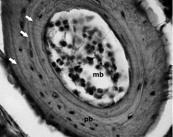
Fig. 1 Examples of phalangeal cross-sections (10 μm thick) of Boana cordobae. Male, SVL: 50.36 mm; 3- year-old. White Arrows = lines of arrested growth (LAGs); mc = medullar cavity; pb = periosteal bone.
Sexual variation in adult age and morphometric variables: Pearson correlation showed that age and most of the measured morphometric variables are correlated (P < 0.05) (only three do not correlate with age: ESD (r = 0.14, P = 0.22), END (r = 0.19, P = 0.09) and RND (r = -0.10, P = 0.36). Differences between males and females were compared by general linear models (GLMs, with age as a covariate). From the 15 variables measured, 13 showed differences between the sexes (P < 0.05). Females were larger than males, except in END (F78 = 2. 15, P = 0.12) and RND (F78 = 0.31, P = 0.58). This too confirm with the sexual dimorphism index (SDI) in body size of 0.095. In specimens of age 2 - 3 - 4 and 7 years, where sample size allowed estimation, variation in SDI was (age of specimens/SDI): 2/0.09, 3/0.08, 4/0.17, 7/0.04 SVL; females were larger than males in average SVL for all ages.
Because the low number of females, and that most of the variables shown significant difference between males and females, later analyzes were carried out only by taking account of the males.
Age and morphometric variables relationships: The variance of the age class in SVL, and in all variables, was the largest in three-year-old males, with a range of 13.88 mm and a standard deviation of 3.54 mm (SVL = 49.84 ± 3.54 mm); and the smallest reproductive male was 41.30 mm. Body length (SVL) showed considerable variation within some age groups, however age and body size were correlated (r = 0.38, P = 0.0017). Largest individuals were almost always the oldest ones. The same was observed for most of the morphometric variables (only three variables were not correlated with age, ESD: r = 0.19, P = 0.1089; ID: r = 0.22, P = 0.08; RND: r = -0.15, P = 0.22).
Altitudinal variation in adult males, age and morphometric variables: Pearson correlation show that age and altitude are not correlated (r = 0.03, P = 0.78) (Table 1). However, average age differs significantly among the six populations (GLMMs F66 = 4.17, P < 0.05), and post-hoc multiple comparisons indicated that he population of at lower altitudes (808m in elevation) differed with other populations, with older average ages; the populations of intermediates altitudes (930, 1 634, 2 107 m.a.s.l) do not differ among them, but with the others, mainly with populations at higher altitudes (2 150 and 2 310 m.a.s.l) (Bonferroni post hoc test, P < 0.05).
Table 1 Means ± standard deviation of age and morphometric variables of adult males of B. cordobae from six populations
| - | Los Linderos 2 310 m.a.s.l. | Pampa de Achala 2 150 m.a.s.l. | Los Tabaquillos 2 107 m.a.s.l. | La Carolina 1 634 m.a.s.l. | Las Guindas 930 m.a.s.l. | Achiras 808 m.a.s.l. |
|---|---|---|---|---|---|---|
| Age | n = 5 | n = 9 | n = 5 | n = 12 | n = 26 | n = 10 |
| - | 4.6 ± 1.82 3-7 | 3.67 ± 0.71 2-4 | 3 ± 1 2-4 | 3.33 ± 1.15 2-6 | 3.27 ± 0.83 2-5 | 4.9 ± 1.45 3-7 |
| SVL | 56.09 ± 2.89 | 49.43 ± 3.32 | 49.59 ± 1.39 | 51.18 ± 3.23 | 47.04 ± 2.51 | 53.43 ± 2.40 |
| HW | 15.91 ± 1.15 | 14.24 ± 0.71 | 15.35 ± 0.61 | 15.02 ± 0.75 | 13.62 ± 0.92 | 15.61 ± 0.75 |
| HL | 17.36 ±1.30 | 15.72 ± 0.76 | 15.57 ± 0.71 | 16.11 ± 1.32 | 14.70 ± 1.14 | 16.61 ± 0.98 |
| ESD | 7.42 ± 0.59 | 6.37 ± 0.43 | 6.80 ± 0.48 | 6.89 ± 0.72 | 6.09 ± 0.59 | 7.23 ± 0.32 |
| IND | 4.55 ± 0.39 | 4.15 ± 0.30 | 4.26 ± 0.22 | 4.20 ± 0.39 | 3.70 ± 0.39 | 4.43 ± 0.25 |
| ID | 5.8 ± 0.53 | 5.02 ± 0.28 | 5.27 ± 0.41 | 5.55 ± 0.42 | 5.45 ± 0.77 | 5.76 ± 0.48 |
| END | 4.47 ± 0.43 | 4.15 ± 0.11 | 3. 93 ± 0.37 | 4.27 ± 0.52 | 3.57 ± 0.45 | 4.22 ± 0.33 |
| RND | 3.28 ± 0.23 | 2.79 ± 0.46 | 3.24 ± 0.55 | 3.32 ± 0.53 | 3.16 ± 0.43 | 3.39 ± 0.36 |
| ED | 5.86 ± 0.45 | 5.09 ± 0.29 | 4.86 ± 0.10 | 4.82 ± 0.47 | 5.07 ± 0.36 | 5.52 ± 0.26 |
| AL | 27.84 ± 0.94 | 24.46 ± 1.27 | 22.74 ± 0.86 | 24.48 ± 1.98 | 22.21 ± 1.80 | 25.91 ± 1.55 |
| FL | 28.75 ± 0.84 | 25.84 ± 1.18 | 25.77 ± 0.80 | 26.37 ± 1.27 | 23.29 ± 1.93 | 28.18 ± 1.37 |
| TL | 27.81 ± 1.02 | 24.94 ± 1.46 | 24.71 ± 0.69 | 25.86 ± 1.50 | 23.89 ± 1.86 | 28.02 ± 1.36 |
| FoL | 37.54 ± 4.93 | 35.71 ± 1.79 | 35.24 ± 2.28 | 36.59 ± 2.04 | 33.31 ± 3 | 38.49 ± 1.27 |
| TF | 12.49 ± 0.70 | 10.68 ± 0.75 | 9.46 ± 1.27 | 10.31 ± 1.17 | 9 ± 0.92 | 11.05 ± 0.72 |
| LF4 | 17.12 ± 1.13 | 16.08 ± 1.57 | 13.26 ± 1.61 | 14.34 ± 2.39 | 12.41 ± 1.38 | 14.80 ± 1.18 |
When the effect to age was controlled, partial correlation show that six morphometric variables were not correlated with altitude (ESD: r = 0.24, P = 0.05; ID: r = - 0.15, P = 0.25; RND: r = - 0.16, P = 0.19; ED: r = 0.0035, P = 0.98; TL: r = 0.14, P = 0.26; FoL: r = 0.21, P = 0.09); while nine were positively correlated with altitude of each population (SVL, HW, HL, IND, END, AL, FL, TF, LF4: P ≤ 0.05), indicating a clinal trend: males at higher altitudes are significantly larger than those at lower altitudes.
The results of PCA indicate that the first three principal components explain 76.64 % of the variation in the original variables, since the three components showed eigenvalues greater or equal to 1.0. PC1 catches mostly variation in measurements concerning to measures related to the body (SVL, HW, HL, AL, FL, TL, FoL, TF, LF4) and the width and length of the head (HW, HL, END), whereas PC2 (RND, ED) and PC3 (ESD, IND, ID) reflects variation in the other variables related to the head (factor loadings summarized in Table 2).
Table 2 Principal component analysis. Factor loading matrix in the first three components
| - | - | Eigenvectors | - |
|---|---|---|---|
| Endpoints | PC1 (61.23 %) | PC2 (8.42 %) | PC3 (6.99 %) |
| SVL | 0.31* | -0.02 | 0.06 |
| HW | 0.29* | 0.05 | 0.03 |
| HL | 0.27* | -0.16 | -0.19 |
| ESD | 0.25 | 0.27 | -0.28* |
| IND | 0.25 | 0.14 | -0.36* |
| ID | 0.13 | 0.34 | 0.73* |
| END | -0.19 | 0.24* | -0.09 |
| RND | 0.05 | 0.75* | -0.30 |
| ED | 0.21 | 0.32* | 0.13 |
| AL | 0.30* | -0.09 | 0.04 |
| FL | 0.31* | -0.051 | 0.04 |
| TL | 0.30* | -0.01 | 0.21 |
| FoL | 0.29* | -0.06 | 0.21 |
| TF | 0.29* | -0.16 | -0.07 |
| LF4 | 0.25* | -0.22 | -0.12 |
The asterisk indicates variables that most strongly correlated with respective principal component.
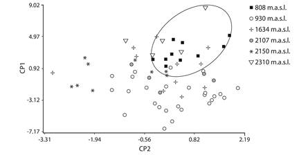
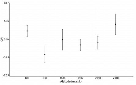
The six studied populations differ significantly in factor scores of PC1 as well as PC2 (GLMs, P = < 0.001). Figure 2 shows that PC1 separates mainly the populations at higher and lower altitudes (2 310 m elevation and 808 m elevation), and post-hoc tests revealed that males of these two populations were larger than the other populations, and at intermediate altitudes (930, 1 634, 2 150 and 2 107 m elevation) the males do not differentiate between them, similar in size (with intermediate values) (Fig. 3). In the PC2 also showed the populations at higher and lower altitudes revealed bigger males, but 2 150 m elevation populations were significantly smalls (Post hoc test Bonferroni, P < 0.001).
Discriminant analysis generated three functions, the first highly significant (P < 0.0001) accounted for 55.19 % of the total variation. Although there was some overlap among populations, when grouping all individuals 74.24 % were correctly assigned to their original population, and in general classification into incorrect was relatively low, except from populations of La Carolina (1 634 m.a.s.l.) (Table 3).
Table 3 Discriminant function analysis. Percentage of correctly classified
| - | - | - | - | - | Clasification table | - | - | - | |
|---|---|---|---|---|---|---|---|---|---|
| Function | 1 | Actual group | n | 808 | 930 | 1 634 | 2 107 | 2 150 | 2 310 |
| Eigenvalue | 1.82 | 808 | 10 | 7 (70 %) | 0 (0.00 %) | 2 (20 %) | 0 (0.00 %) | 1 (10 %) | 0 (0.00 %) |
| Relative % | 55.19 | 930 | 26 | 0 (0.00 %) | 21 (80.77 %) | 3 (11.54 %) | 2 (7.69 %) | 0 (0.00 %) | 0 (0.00 %) |
| Canonical correlation | 0.80 | 1 634 | 11 | 1 (9.09 %) | 1 (9.09 %) | 5 (45.45 %) | 1 (9.09 %) | 2 (18.18 %) | 1 (9.09 %) |
| Wilk´s lambda | 0.11 | 2 107 | 5 | 1 (20 %) | 0 (0.00 %) | 0 (0.00 %) | 4 (80 %) | 0 (0.00 %) | 0 (0.00 %) |
| X2 | 126.11 | 2 150 | 9 | 0 (0.00 %) | 0 (0.00 %) | 1 (11.11 %) | 0 (0.00 %) | 8 (88.89 %) | 0 (0.00 %) |
| df | 45 | 2 310 | 5 | 0 (0.00 %) | 0 (0.00 %) | 1 (20 %) | 0 (0.00 %) | 0 (0.00 %) | 4 (80 %) |
| P | 0.0000 | - | - | - | - | - | - | - | - |
Discusion
This study shows that: 1) the age differs significantly among the six populations of Boana cordobae, and as morphometric variables positively correlates to age, this age differences can partly explain the geographic variation of morphometric variables; 2) ageadjusted morphometric variables allow that differences among sites became more significant; 3) the patterns of variation in age and morphometric variables are related with the climate, and therefore this could be related to Bergmann’s rule.
The presence of growth layers in bone tissue and counting the lines of arrested growth (LAGs) serve to evaluate age in B. cordobae (Otero et al., 2017a) and our study confirm that scheletochronology works well for age determination in the species.
Sexual size dimorphism is well known in most anurans (Mao et al., 2012; Liu et al., 2012; Lou et al., 2012; Otero et al., 2017b). In this study, there was a significant difference in most morphometric variables between sexes, even when the effect of age was removed, confirming the results of past studies on this species (Otero et al., 2017a). There is a marked sexual dimorphism; adult females are significantly larger than adult males. Numerous factors can explain sexual dimorphism in B. cordobae have been reported by these authors.
In our study, the relationship between age and several morphometric variables confirm similar results reported for this species (Otero et al., 2017a), where anurans exhibit indeterminate growth, implying that body size increases with age (Halliday & Verrell, 1988; Duellman & Trueb, 1994). Since body size can reflect individuals age in anurans (Liao & Lu, 2010; Ashkavandi et al., 2012; Altunişik and Özdemir, 2013; Otero et al. 2017a; Otero et al., 2017b) age is key as a covariate in morphometric studies.
Our results demonstrated that populations of B. cordobae vary in morphometric variables. We found a clinal trend in the morphometric variables: populations inhabiting different altitudes showed that individuals from higher altitudes were larger than those from lower altitude. In ectothermic animals with indeterminate growth, such as most amphibians, adult body size can show intra-specific geographic variation, because associations between an organism’s size and its environment (Angilletta & Dunham, 2003; Morrison & Hero, 2003; Rosso, Castellano, & Giacoma, 2004). It is expected that organisms exhibit larger adult size in colder environments (Partridge & French, 1996; Ashton, 2002; 2004; Lu et al., 2006), relation that even holds when altitude or latitude is used as a proxy for environmental temperature (Ashton, 2002; Angilletta & Dunham, 2003; Gül, Özdemir, Üzüm, Olgun, & Kutrup, 2011; Altunişik and Özdemir, 2013). This fact is due cold temperatures retard both growth and development, and therefore individuals mature after and consequently the adults are larger and/or older (Morrison, Hero, & Browning, 2004; Rosso et al., 2004). As a result, high-altitude amphibians commonly are larger than those of low-altitude (Miaud et al., 1999; Iturra-Cid et al., 2010; Liao & Lu, 2010; Hsu, Hsieh, Hu, & Kam, 2014; Altunışık & Özdemir, 2015), the so-called Bergmann’s rule.
Our data show that the highest values of morphometric variables and maximum life span were observed in the two populations with the higher altitude and the lower altitude, Los Linderos (2 310 m elevation) and Achiras (808 m elevation). Furthermore, the ages (average age and longevity; Table 2) of specimens of these sites were higher than those from other populations. These results are noteworthy, because the morphometric variables and age are expected to be higher in highland populations as shown by other studies (Lai et al., 2005; Liao & Lu, 2010). Although part of our results confirms this trend, in this study, also average morphometric variables and age of the lowest population were higher. This fact shows that there are exceptions to the Bergmann’s rule, with individuals in lowland population being significantly larger and older. Some authors associated these exceptions with parameters having effects on body size such as food availability, habitat quality, competition, and predation pressure on age at maturity, and limited altitudinal gradients (e.g.; Morrison & Hero, 2003). We believe that, individuals from Achiras were larger and older than in other populations due the characteristics of the site where there live. Individuals were collected in water bodies associated to the river of a tourist locality, with presence of artificial light at night which favors the food availability and a longer growing season (personal communication). These same explanations were proposed by Liao et al. (2010b) when individuals of Rana nigromaculata from low altitudes were larger and older than those of higher sites.
In the results presented by Baraquet et al. (2012), individuals from Las Guindas (930 m elevation) showed lowest values in all morphometric variables and differing significantly from the other populations. However, in this paper age was not used as covariate. When age was included as a covariate, the posteriori test showed that the populations with higher differences were the sites with the higher altitude and the lower altitude, Los Linderos and Achiras. Thus, because body size may be a consequence of differences in age (Castellano & Giacoma, 2000), including individuals age improves significantly the results of studies evaluating morphometric variables (Kupfer, 2009).

