


 Inglês (pdf)
 Artigo em XML
 Referências do artigo
 Enviar este artigo por email
 Citado por SciELO
  Similares em
SciELO
Similares em
SciELO  uBio
uBio 
 Permalink
Ecosystems are subject to intense anthropic pressure, with agriculture being mainly responsible for the modification of small streams in rural areas (Conroy et al., 2016). In these areas, landscape modification directly threatens streams, especially due to the removal of riparian vegetation (Allan, 2004; Johnson & Almlöf, 2016). As a result of the removal of this vegetation, there is an increase in the supply of agrochemicals, nutrient enrichment and contamination by metals in streams (Foley et al., 2005; Woodward et al., 2012). Therefore, anthropic impacts modify geomorphic processes that maintain the aquatic landscape and its biota (Taroli & Sofia, 2016). Lotic ecosystems are altered at various spatial scales (Allan, 2004), leading to the simplification of water bodies (Bleich, Mortati, André, & Piedade, 2014) and the dominance or exclusion of certain organisms (Greenwood, Harding, Niyogi, & McIntosh, 2012).
In undisturbed communities of organisms, species have a distinct distribution (Heino & Mendoza, 2016), where some species are very abundant, others only moderately common, while the rest of the species are rare. Species may be biologically distinct in various ways, such as in relation to their dispersal ability and life strategies (Roque et al., 2016). Therefore, species may respond differently to environmental conditions (Hepp, Landeiro, & Melo, 2012; Heino & Mendoza, 2016) and spatial processes (Kunin & Shimida, 1997; Cornwell & Ackerly, 2010; Hepp & Melo, 2013).
In the conservation context, the importance of rare organisms within aquatic communities has been much discussed (Heino & Mendoza, 2016; Roque et al., 2016) and various approaches are used to incorporate the rarity of species into analyses (Siqueira et al., 2011). On the other hand, these organisms can be considered as the best indicators of environmental stress (Poos & Jackson, 2012). Therefore, the exclusion of rare organisms in the original matrices requires good justification, since the results obtained can be drastically divergent (Poos & Jackson, 2012).
The dissimilarity of aquatic communities can be influenced by environmental or spatial factors. Limnological factors are related to local effects that act directly on organisms (Hepp et al., 2012). On the other hand, spatial factors act on the dispersal potential of organisms (Hepp & Melo, 2013). The effects of limnological variables and characteristics of land use are more easily perceived than spatial factors, since they act on organisms at smaller scales (Sensolo, Hepp, Decian, & Restello, 2012; Hepp, Milesi, Biasi, Restello, & Molozzi, 2013; Ferreira et al., 2017). The identification of the main factors that control the structuring of the communities increases our knowledge of the distribution patterns of the species therein, and consequently assists in decision making for environmental conservation and recovery programmes (Vinson & Hawkins, 1998).
In this study, we evaluated the influence of limnological variables and land use in the upper Uruguay river drainage basin on the assemblage composition of the orders Ephemeroptera, Plecoptera and Trichoptera (EPT). We used different biological matrices (total genera, common genera only, and rare genera only from the EPT assemblages) in order to verify their relationship with the environmental variability observed in small-order streams. Our hypothesis is that the environmental matrix will have a significant relation with the biological matrix composed by the common genera of EPT. We believe that this will happen, since the structuring of communities is usually done by common species. In addition, we predict that the rare genera will contribute little to the dissimilarity of the assemblages, presenting relationships with similar environmental variables.
Materials and methods
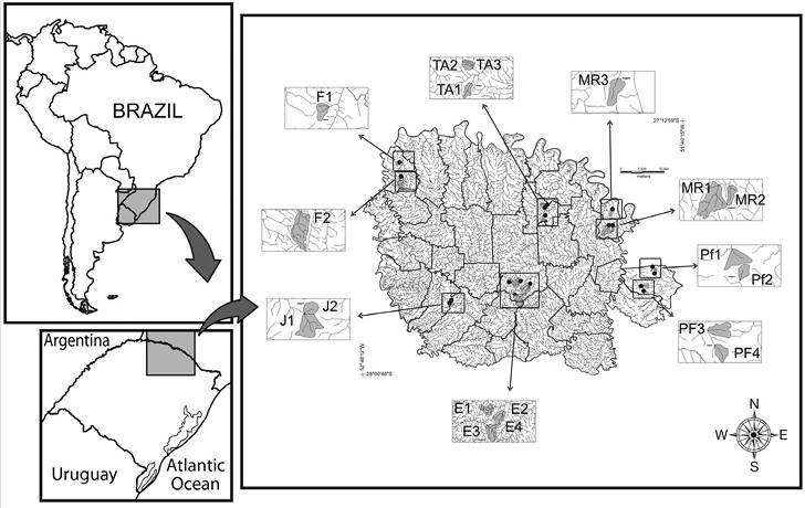
Study area: We conducted this study in 18 streams located in the Atlantic Forest, in southern Brazil (Figure 1). The vegetation of the study region is characterised by a transition zone between perennial seasonal forest with Araucariaand seasonal semideciduous forest (Oliveira-Filho, Budke, Jarenkow, Eisenlohr, & Neves, 2015). The climate is subtropical of the temperate type (type Cfb of Köppen classification), with an average annual temperature of 17 ± 1 ºC and average annual rainfall that varies between 1 900 and 2 200 mm (Alvares, Stape, Sentelhas, Gonçalves, & Sparovek, 2013). The area is intensely fragmented; approximately 20 % of the area is covered with native tree vegetation, while the rest of the area is occupied by agricultural and urban activities (Decian, Zanin, Oliveira, & Rosset 2010).
Land use analysis: For the landscape analysis we calculated the percentages of land uses (images 1:25 000) using the buffer area defined by a 30 m extension of both banks of the streams. We calculated the buffer areas of each of the 18 streams following the cartographic parameters of selection of the quoted points and the water dividers. For this purpose we used the software MapInfo 8.5 and Idrisi 32. The cartographic base adopted for the work was of the scale 1:35 000 and ETM + sensor image of Landsat 7 satellite of the year 2005, with a spatial resolution of 15 m and spectral bands 3, 4, 5 and panchromatic. The quantification of landscape attributes was defined according to the cartographic parameters of selection of water bodies and the use of Boolean, distance and context operations of GIS applications. Land use classification followed the method of Maximum Likely Supervision in the SIG IDRISI 32, based on sample units obtained in the field using GPS, with prior knowledge of the area. The classes adopted for the work were agriculture, exposed soil, pasture and vegetation.
Limnological variables: In the selected streams, we measured water temperature, electrical conductivity, pH and dissolved oxygen using a multiparameter analyser Horiba® U55. At the same sites we collected water samples for quantification of dissolved organic carbon (DOC) and total nitrogen using a Shimadzu® TOC-VCSH Analyser. We also measured the concentration of sulphate ions using a High Performance Liquid Chromatography. The analytical methodologies are described in Standard Methods (APHA, 1998).
Sampling of stream insects: We collected the aquatic insects in March 2010 using a Surber sampler (area of 0.09 m2) and a mesh size of 250 μm. The streams were of the first and second order with widths of approximately 1.5-2 m, depth less than 0.3 m and the presence of rapids and stony substratum. The material collected was fixed in the field with 80 % ethanol, packed in plastic containers and taken to the laboratory. Later, they were identified to genus level, according to the keys of Salles, Da-Silva, Serrao, and Francischetti (2004), Pes, Hamada, and Nessimian (2005), and Mugnai, Nessimian, and Baptista (2010).
Data analysis: We used the percentages of relative abundance proposed by Siqueira et al. (2011) as the criteria of rarity. Taxa with relative abundance values below in the first three quartiles were considered to be rare genera, whereas organisms with relative abundance in the fourth quartile were considered to be abundant genera. Using this distinction, we analysed a biological matrix of all identified genera (total matrix), a matrix of only abundant genera (common matrix) and a matrix of only rare genera (rare matrix).
The matrices were transformed (log [x + 1]) to guarantee the homoscedasticity of the data. To verify the correlation between dissimilarity matrices (Bray-Curtis dissimilarity) and environmental variables (which included those related to land use) we used a BioENV analysis (Clarke & Ainsworth, 1993). We used a Mantel test to verify the significance of the correlations between the best models with the dissimilarity of the biological matrices. The analyses were performed in the statistical program R (R Core Team, 2014), using functions of the “vegan” package (Oksanen et al., 2014).
Results
Environmental characterisation: The 18 studied streams showed wide environmental variability, both regarding land use and limnological characteristics (Table 1). The water temperature varied between 19.9 and 27.7 °C and was well oxygenated (7.0-9.3 mg L-¹). The pH remained between neutral and slightly basic (7.1-9.1) and the electrical conductivity was low (0.01-0.11 mS cm-¹). The DOC varied between 6.73 and 335.3 mg L-¹, while total nitrogen varied between 1.0 and 6.1 mg L-¹. Among the land use classes, agriculture accounted for 1.97-44.3 % of the area around the streams, pasture comprised 0-34.5 %, exposed soil accounted for 1.0-34.2 %, and vegetation covered 0-15.9 % of the area (Table 2).
Table 1: Physic-chemical variables measured in streams studied in Southern Brazil
| Streams | T (˚C) | DO (mg L -1 ) | pH | EC (mS cm -1 ) | DOC (mg L -1 ) | TN (mg L -1 ) | SO 4 (mg L -1 ) |
|---|---|---|---|---|---|---|---|
| E1 | 24.3 | 8.0 | 8.8 | 0.08 | 14.6 | 2.5 | 0.26 |
| E2 | 27.8 | 8.4 | 8.8 | 0.11 | 17.8 | 3.8 | 0 |
| E3 | 20.3 | 7.9 | 8.4 | 0.05 | 9.6 | 1.5 | 0.25 |
| E4 | 20.8 | 8.8 | 8.4 | 0.07 | 40.4 | 3.0 | 0.38 |
| TA1 | 24.3 | 6.5 | 8.3 | 0.11 | 63.4 | 5.8 | 1.08 |
| TA2 | 21.4 | 9.3 | 8.3 | 0.11 | 24.7 | 5.4 | 1.58 |
| TA3 | 22.3 | 5.4 | 8.0 | 0.10 | 30.2 | 3.7 | 1.22 |
| F1 | 21.7 | 7.9 | 7.7 | 0.02 | 335.3 | 1.2 | 0.25 |
| F2 | 21.1 | 8.0 | 7.1 | 0.01 | 19.5 | 1.2 | 0.13 |
| PF1 | 21.5 | 8.7 | 8.5 | 0.11 | 27.4 | 4.5 | 0.88 |
| PF2 | 22.1 | 9.2 | 8.3 | 0.07 | 37.5 | 6.1 | 0.82 |
| PF3 | 22.5 | 7.2 | 8.3 | 0.07 | 19.3 | 1.5 | 0.49 |
| PF4 | 24.6 | 8.2 | 9.1 | 0.08 | 34.8 | 3.3 | 0.83 |
| MR1 | 19.9 | 8.6 | 8.2 | 0.08 | 59.2 | 1.0 | 0.72 |
| MR2 | 21.3 | 8.0 | 8.2 | 0.09 | 77.8 | 1.2 | 0.76 |
| MR3 | 19.9 | 8.7 | 8.1 | 0.09 | 92.5 | 2.3 | 0.25 |
| JAC1 | 22.0 | 7.1 | 7.7 | 0.02 | 6.7 | 2.3 | 0.17 |
| JAC2 | 23.3 | 6.8 | 7.9 | 0.03 | 16.4 | 3.0 | 0.27 |
T: water temperature, DO: dissolved oxygen, pH: water pH, EC: electrical conductivity, DOC: dissolved organic carbon, TN: total nitrogen, SO4: sulfate.
Table 2: Land uses measured in the buffer zone (30 m) in the streams studied in Southern Brazil
| Streams | Agriculture (%) | Pasture (%) | Exposed soil (%) | Riparian Vegetation (%) |
|---|---|---|---|---|
| E1 | 23.7 | 30.7 | 7.5 | 10.4 |
| E2 | 25.2 | 34.5 | 18.5 | 10.1 |
| E3 | 9.0 | 1.2 | 8.4 | 4.8 |
| E4 | 31.7 | 26.4 | 34.2 | 15.9 |
| TA1 | 2.0 | 0.1 | 1.2 | 8.6 |
| TA2 | 7.9 | 2.6 | 6.7 | 10.3 |
| TA3 | 7.9 | 0.1 | 3.9 | 11.6 |
| F1 | 22.6 | 11.3 | 33.2 | 15.2 |
| F2 | 3.6 | 2.8 | 2.1 | 3.7 |
| PF1 | 5.3 | 0 | 3.5 | 13.9 |
| PF2 | 7.7 | 0 | 8.9 | 6.5 |
| PF3 | 1.9 | 0 | 4.4 | 1.2 |
| PF4 | 3.8 | 0 | 12.3 | 1.0 |
| MR1 | 10.3 | 0.2 | 3.1 | 2.9 |
| MR2 | 44.3 | 4.1 | 10.2 | 14.2 |
| MR3 | 10.1 | 0 | 1.0 | 2.7 |
| JAC1 | 2.7 | 0.4 | 2.0 | 0.4 |
| JAV2 | 5.5 | 4.4 | 10.6 | 0 |
EPT assemblages: We collected a total of 6 023 organisms, distributed among 41 genera. Trichoptera was the most abundant order (3 748 individuals, 16 genera), followed by Ephemeroptera (1 931 individuals, 20 genera) and Plecoptera (344 individuals, 5 genera). The matrix with the common genera represented 86 % of the total abundance divided into only 10 genera. The three most abundant genera were the caddisfly Smicridea (Hydropsychidae, 44.9 % of the total abundance), Metrichia (Hydroptilidae, 14.4 %) and the mayfly Farrodes (Leptophlebiidae, 12 %). Rare genera totalled 384 individuals (6.4 % of the total abundance) and were represented by 31 genera. The number of rare genera identified accounted for 75 % of the taxonomic richness.
Assemblage dissimilarity: We not observed correlation between the physical-chemical and land use matrices (r = 0.23, P = 0.18). The dissimilarity of the total EPT matrix and the common genera matrix were correlated with pH, electrical conductivity, native tree vegetation and exposed soil (r = 0.51, P = 0.02 and r = 0.53, P = 0.004, for the total and common matrices respectively; Table 3). On the other hand, the dissimilarity of the rare EPT matrix was correlated with pH, electrical conductivity and native tree vegetation (r = 0.48, P = 0.03; Table 3).
Table 3: BioEnv analysis, correlation of the rare EPT matrix (using the rare organisms from the assemblages of EPT collected in the streams) associated with the environmental matrix in the streams studied
| Total EPT | Correlation |
| pH | 0.37 |
| pH + Veg | 0.49 |
| pH + EC + Veg | 0.50 |
| pH + EC + Soil + Veg | 0.51* |
| pH + EC + TOC + Soil + Veg | 0.49 |
| pH + EC + TOC + SO4 + Soil + Veg | 0.47 |
| pH + EC + TOC + SO4+ Past + Soil + Veg | 0.43 |
| pH + EC + TOC + TN + SO4+ Past + Soil + Veg | 0.39 |
| T + pH + EC + TOC + TN + SO4+ Past + Soil + Veg | 0.34 |
| T + pH + EC + TOC + TN + SO4+ Agri + Past + Soil + Veg | 0.30 |
| T + DO + pH + EC + TOC + TN + SO4+ Agri + Past + Soil + Veg | 0.27 |
| Common EPT | |
| pH | 0.37 |
| pH + Veg | 0.48 |
| pH + Soil + Veg | 0.52 |
| pH + EC + Soil + Veg | 0.53* |
| pH + EC + TOC + Soil + Veg | 0.51 |
| pH + EC + TOC + Past + Soil + Veg | 0.49 |
| pH + EC + TOC + SO4+ Past + Soil + Veg | 0.45 |
| pH + EC + TOC + SO4+ Agri + Past + Soil + Veg | 0.41 |
| T + pH + EC + TOC + SO4+ Agri + Past + Soil + Veg | 0.36 |
| T + DO + pH + EC + TOC + SO4+ Agri + Past + Soil + Veg | 0.31 |
| T + DO + pH + EC + TOC + TN + SO4+ Agri + Past + Soil + Veg | 0.25 |
| Rare EPT | |
| EC | 0.38 |
| pH + Veg | 0.46 |
| pH + EC + Veg | 0.48* |
| pH + EC + TN + Veg | 0.45 |
| pH + EC + TOC + TN + Veg | 0.45 |
| pH + EC + TOC + TN + SO4 + Veg | 0.41 |
| pH + EC + TOC + TN + SO4 + Agri + Veg | 0.37 |
| pH + EC + TOC + TN + SO4 + Agri + Soil + Veg | 0.33 |
| T + pH + EC + TOC + TN + SO4 + Agri + Soil + Veg | 0.27 |
| T + DO + pH + EC + TOC + TN + SO4 + Agri + Soil + Veg | 0.21 |
| T + DO + pH + EC + TOC + TN + SO4 + Agri +Past + Soil + Veg | 0.16 |
EC: Electrical conductivity, pH: Water pH, DO: Dissolved oxygen, TN: Nitrogen, TOC: Total organic carbon, SO4: Sulfate, Veg: Vegetation, Agri: Agriculture, Soil: Exposed soil, Past: Pasture. *Best model.
Discussion
The EPT assemblages contained few common genera and many rare genera. In unequal communities, the most abundant species maintain their ecological conditions, on the other hand, the species little abundant, lose resources (e.g. food, habitat), becoming rare (Tokeshi, 1990). This is expected for most aquatic communities because in these ecosystems, patterns of distribution of abundance and composition are the result of the interaction between species behaviour, physical conditions of the habitat (e.g. substrate, stream, riparian vegetation) (Hepp et al., 2012; Ferreira et al., 2017), and limnological parameters (e.g. temperature, nutrients, turbidity) (Hepp et al., 2013).
In this study, the same environmental variables were related to the dissimilarity of common and rare genera. This demonstrates that dominant organisms structure communities, even with environmental variability. In addition, rare taxa did not show a higher level of environmental specialisation when compared to common genera; however, rare genera can be affected by variables that are difficult to measure, particularly biotic factors (Siqueira et al., 2011). Rare species have restricted spatial distribution as well as low density (Fontana, Ugland, Gray, Willis, & Abbiati, 2008). According to Reichert et al. (2010), there is a significant increase in assemblage richness across spatial scales, which is important for beta diversity in a particular region (Clarke, MacNallym, Bond, & Lake, 2008). However, the occurrence of rare species can be affected by environmental heterogeneity (Clarke et al., 2008), dispersion limitation (Malmqvist, 2002) and environmental fragmentation (Fagan, Unmack, Burgess, & Minckley, 2002).
All biological matrices studied here showed the dependence with water pH, electrical conductivity and percentage of native tree vegetation in adjacent areas. In aquatic ecosystems, pH is a regulating variable of local aquatic fauna, as changes in the pH of streams may be responsible for changes in the levels of toxicity of heavy metals (Hall, Likens, Fiance, & Hendrey, 1980). In turn, riparian vegetation plays an important role in small streams. Riparian vegetation provides coarse particulate matter to streams and increases habitat heterogeneity with leaf, branch and fruit entry (Gonçalves, Rezende, Grégori, & Valentin, 2014). This habitat heterogeneity allows a greater number of individuals to settle in a certain place, since in addition to food supply, the habitat also provides shelter to aquatic organisms (Graça et al., 2004). Hepp et al. (2012) cite that environmental variables such as substrate heterogeneity and particulate organic matter content are environmental factors that exert more prominent effects on aquatic invertebrates than the spatial position of streams. In addition, the increase of exposed soil in areas adjacent to small streams causes an increase in the sediment input to the stream (Wantzen & Mol, 2013). Because they are areas where agricultural practices are carried out, the entry of agricultural fertilisers and pesticides residues associated with the sediment potentially increases the concentration of nutrients dissolved in the streams (Sensolo et al., 2012).
In this study, the common genera were important in the structural patterns of the EPT assemblages in the streams studied. The variation in the amount of exposed soil in the study area was correlated with the common genera and the changes to the total EPT assemblage that occur in the areas adjacent to the streams. Large areas of exposed soil alter the entry of organic matter and increase the input of sediment to the streams. The changes in the availability of dissolved organic material are strongly associated with common taxa. In addition, the presence of riparian vegetation on the streams was important for the three EPT matrices studied, reinforcing the dependence of these organisms on the conservation of aquatic environments. The riparian vegetation was an important environmental factor that generated the dissimilarity of the communities. Many organisms are dependent on the input of allochthonous organic matter that serves as a source of food or shelter (Hepp et al., 2016).
In summary, in our study we corroborate the importance of riparian vegetation for aquatic communities in streams, acting as a source of food resource and refuge (Sensolo et al., 2012; Ferreira et al., 2017). In addition, the variability of EPT assemblages was associated with pH, electric conductivity, exposed soil, and riparian vegetation. This showed that the environmental factors environmental factors can structure communities at different scales (stream or riparian zone). Thus, strategies and programs for the conservation of aquatic biodiversity should not only observe local scales for conservation, including wider scales (e.g. landscape).

