


 Espanhol (pdf)
 Artigo em XML
 Referências do artigo
 Enviar este artigo por email
 Citado por SciELO
  Similares em
SciELO
Similares em
SciELO 
 Permalink
Introduction
X-rays are widely used in industry, engineering, health sciences and other areas for applications such as material characterization, analysis of fatigue and fractures in materials, and medical diagnostic or therapeutic purposes (Bilge, 2004; Carrera et al., 2019; Durán-Nava et al., 2019; Epp, 2016).
The energy and intensity of the X-ray beam employed differs for each application. In medical diagnostic and therapy, superficial X-rays ranging from approximately 50 to 250 keV are used to produce images of different parts of the body or to treat skin cancers (Hill et al., 2014; Tafti & Maani, 2020). The contrast of the radiographic image, as well as the delivered dose to the patient, depend critically on the X-ray energy spectrum. The spectrum can be also important to characterize the dosimetric properties of the beam (Chen et al., 2012), for quality control of mammography equipments and x-ray tubes (Abbene et al., 2012; Maeda et al., 2005; Querol et al., 2010), and optimization of image quality parameters (Malezan et al., 2015).
The X-ray production is commonly influenced by the tube’s peak potential (kVp), electronic current (mA), anode material and filtration (Nakashima & Duong, 2020; Sharma et al., 2015; Tafti & Maani, 2020; Thunthy & Manson-Hing, 1978). The energy spectrum of an X-rays beam is defined as the energy distribution of the produced photons (Nickoloff & Berman, 1993; Tafti & Maani, 2020).
Experimental, computational, or mathematical methods can be used to as-method can be used to computationally simulate the produced X-rays. Mathematical methods usually derive the spectrum from experimental transmission curves of the X-rays by a given material (Chen et al., 2012; Hill et al., 2014).
Some difficulties of experimental and computational approaches are related to the cost of the spectrometer, specific information about the geometry and materials of the X-ray equipment for use in the Monte Carlo modelling (Baird, 1981; Hill et al., 2014) and expertise (Menin et al., 2016). Furthermore, softwares as SpekCalc only allow calculations for a fixed source-detector distance (Poludniowski et al., 2009).
In the present work, transmission curves are used to obtain the energy spectra from a clinical orthovoltage equipment. Inverse Laplace transform of the transmission data (Benjamin R. Archer & Wagner, 1988) is employed along with the generalized simulated annealing (Wilches Visbal & Da Costa, 2019).
Methodology
Mathematical modelling
In radiation physics it is possible to related the air collision kerma Kcol to the energy distribution fluence of a photon beam Φ (E) as (Menin et al., 2016),
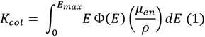
where  is the mass absorption coefficient for photons with nominal ener-gy E, and Emax the maximum energy of the beam, determined by the voltage peak of the X-ray tube.
For a narrow beam, the attenuated energy distribution fluence obtained as an X-ray beam traversed an absorber material of thickness x is,

where Φ 0(E) is the non-attenuated energy distribution fluence of the beam (x = 0) and µm is the mass attenuation coefficient of the absorber, which is a function of E.
Substituting eq. (2) in (1), the Kcol for an attenuated X-ray beam is,

meanwhile for a non-attenuated beam is, the K air is

From eq. (3) and (4) the relative transmission is obtained as,

or also,

where Kcol,0 is obtained from an ionization chamber reading without absorber and Kcol,x is the reading with an absorber of thickness x between the X-ray source and the detector, considering the influence variables (e.g., temperature and pressure) and calibration coefficient of the detector (Smith, 2000).
Considering that (Pamplona & Costa, 2010)

and substituting eq. (7) in eq. (5)

Changing the integration variable from E to µm”

eq. (8) becomes,

assuming that µm is a monotonic and decrescent function with the energy. As eq. (10) complies with the definition of Laplace transform (L) (B. Archer & Wagner, 1982),

If the transmission curve is known, then ƒ(µm)is obtained by the inverse Laplace transform,

So, the energy spectrum can be determined as (B. R. Archer et al., 1985; B. Archer & Wagner, 1982)

Math conditions for obtaining the transmission and energy spectrum from eq. (10) and (13) are exposed in B. Archer & Wagner, (1982).
In this work, the best model that for such requirements (B. R. Archer et al., 1985) was assumed, but including characteristic radiation (Benjamin R. Archer & Wagner, 1988). Hence, the transmission over a material of thickness x becomes,

where a, b and v are fitted parameters; µm,0 is the mass attenuation coefficient at the nominal energy of the beam; r is the fraction of the bremsstrahlung component; Ci is the relative abundance of the i-th characteristic X-ray line and µm,i is the respective mass attenuation coefficient.
The energy spectrum of an X-ray beam is given by (Benjamin R. Archer & Wagner, 1988),

function, and d (E - Ei) is the Dirac delta function of the difference between the nominal energy E and the energy of the i-th characteristic X-ray line.
The purpose is to find the a, b and r parameters in the eq. (5) by using an opti-mization function to determine the spec-trum F (E). Benjamin R. Archer & Wagner, (1988) published values of Ci and µm,i. For
finding the  it is necessary to fit µm to a fifth degree polynomial (B. R. Archer et al., 1985).
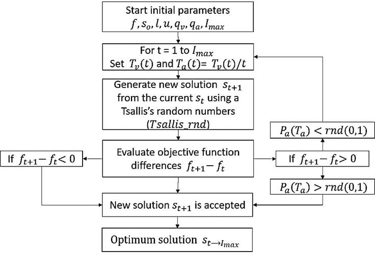
Generalized simulated annealing function (GSA)
To assess the values of a, b and r from eq. (5) it is necessary to use an optimization method for minimizing the residual norm of T(x). Among the existing optimization algorithms, generalized simulated annealing (GSA) is one of most popular and efficient. GSA is a metaheuristic method for solving optimization problems where the global optimum is behind many local minima. GSA mimics the physical annealing, where a metal is heated up to a high temperature for later slowly cooling until reaching a crystalline structure free from imperfection (Wilches Visbal & Da Costa, 2019).
In GSA, there are three important factors for convergence to the global optimum: i) visiting distribution (gv); ii) acceptance probability (Pa), and iii) cooling schedule (Tv). The first factor is related to the achievement of a new solution from the current one; the second factor is associate with an acceptance rule of a new solution, and the third one refers to the capacity of allowance of solutions far from the current one (Deng et al., 2004; Wilches Visbal & Da Costa, 2019).
In a recently work, the GSA function inspired by the generalized simulated annealing algorithm was developed in MATLAB® (Wilches Visbal & Da Costa, 2019). The basic form of the function is:

where s is the solution vector; ƒval is the value of the objective function (functional) ƒ in the solution; so is the initial point; l is the lower bound; u is the upper bound; qu is the visiting parameter, qa is the acceptance parameter, and Imax is the maxi-mum number of iterations.
Figure 1 shows the basic flowchart of the GSA algorithm contained in the GSA function.
Note: derived from research.
Figure 1 Flowchart of the GSA algorithm used in the reconstruction process.
The efficiency of GSA function was tested for optimization problems of varying complexity and has also been used for the assessment of electron beam spectra (Visbal & Costa, 2019).
Reconstruction methodology
The steps for deriving the spectra of X-rays beams are the following (Gonçalves et al., 2020):
Determination of experimental transmission data: X-ray beams from a Siemens Stabilipan-II from Hospital of Clinics at Ribeirão Preto, Brazil, were used to irradiate aluminum plates (purity better than 99 %) of different thicknesses (cm). X-ray beams were adjusted with the inner collimator of the equipment for a field size of 10 x 10 cm2. Thickness of each plate was con-verted to specific thickness (g/cm2) con-sidering the density of aluminum as 2.7 g/cm3. Beams produced at 80 kVp (x = 0.0 cm up to 0.5 cm) and 120 kVp tube voltages (x = 0.0 cm up to 0.7 cm) were used. The aluminum plates were placed at the output window of the equipment.
A Radcal 2086 ionization chamber was used to obtain the air kerma for non-attenuated beams (without plates) and for attenuated (or transmitted) beams (with plates). The distance from the radiation source to the center of ionization chamber was 40 cm. The transmission values were calculated by means of eq. (12).
Calculation of parameters of the transmission T(x): Objective function (T), given by
was minimized employing the GSA function (i.e., g(T) = ƒ in Fig. 1), with qv = 2.7, qa = -5 and Imax = 200. The bounds imposed were 0 < a < 10; 0 < b < 1, 0 < v < 1 and 0 < r <1. Initial point was a vector of random numbers. Imax = 100 for 80 kVp and 300 for the 120 kVp beam.
The stopping condition for the recon-struction algorithm was that the mean square percentage error (MSPE) between experimen-tal transmission data and those from the fitted transmission curve were lower than 1%. The same limit was set to the relative error be-tween the HVL of the transmission curve and the derived one from the spectrum.
Calculation of the F (E): Once the parameters of eq. (15) have been found, they are replaced in eq. (7) for obtaining the spectrum of each X-ray beam. , Г(v) and (E Ei) were computed applying the functions fit, gamma and KronD of MATLAB®. Lastly, the spectrum was obtained by normalizing F (E) to its maximum value.
Validation of the reconstruction methodology was obtained by the comparison between the HVLs from the transmission curves (HVLT(x)) and from the spectra (HVLF(E)), since real (experimental) spectra were not available. HVLF(E) is calculated as,
where Kar,0, Kar,1 and Kar,2 are the air kerma values measured without absorber material (x0 = 0) and with absorber with a thickness immediately lower (x1) and greater (x2) tan the HVL value of the transmission curve, respectively (Gonçalves et al., 2020).
Air kerma of both X-rays beams was computed by utilizing the following equation (Gonçalves et al., 2020),
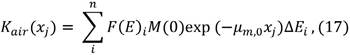
where i = (1, 2, ... n) is the i-th energy beam Ei that makes up the X-ray spectrum, n is the index of the maximum energy beam of photons that makes up the X-ray spectrum; j = (0, 1, 2, .., 5) is the j-th value of the thickness of the absorbing material and DEi the chosen energy interval.
Calculations involved in the recon-struction process were performed with MAT-LAB® 2017a in a personal computer run-ning with Microsoft Windows 10 Pro 64-bit (Core: i7, CPU: 1.8 GHz, RAM: 12 Gb).
Analysis and Results
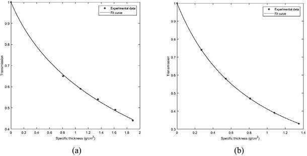
Figure 2 shows the normalized transmission for the 80 kVp (a) and 120 kVp (b)
Note: derived from research.
Figure 2 Transmission of 80 kVp (a) and 120 kVp (b) X-ray beams. Curves were found from minimizing process associated to eq. (15).
X-ray beams. The curves are exponentially decreasing with the thickness of aluminum plates, as expected.
In Table 1 the values of fitted param-eters by means of the minimization process of the functional g(T) are shown.
Table 1 Non-linear fit parameters found from the minimization of the functional (T) for the 80 kVp and 120 kVp X-ray beams.
| Beam energy | a | b | v | r |
| 80 kVp | 3.394 | 0.660 | 0.711 | 0.855 |
| 120 kVp | 7.893 | 0.594 | 0.506 | 0.565 |
Note: derived from research.
The residual norms of eq. (15) were 4.3 x 10⁻⁵ and 1.0 x 10⁻⁴ for the 80 kVp and the 120 kVp beams respectively, whilst the parameters calculation times were 5 sec and 14 sec approximately. The MSPEs were 0.79 % and 0.82 % for the 80 kVp and the 120 kVp beams, respectively. Determination coefficient was greater than 0.99. The good adjustment between transmisión parameters are adequate for assessing the spectra from eq. (13).
Figure 3 shows the normalized energy spectrum of the 80 kVp (a) and 120 kVp (b) X-ray beams obtained by substituting the parameters of Table 1 in eq. (13).
The spectra are right-skewed normal distributions where the peak is the most probable bremsstrahlung energy. The bremsstrahlung component was close to 90% of the total fluence for the 80 kVp beam and approximately 57% for the 120 kVp beam. It is also observed the presence of characteristic X-ray lines in 58, 59.5, 67 and 69 kV, corresponding to the Tungsten-anode K-edge energies. The most probable energy was located at 29.8 keV for the 80 kVp beam and at 40.4 keV for the 120 kVp beam.
For the validation of the reconstruc-tion process, the first HVLs given by the transmission curve and the energy spectrum, were compared. HVLT(x) was computed by inverse interpolation to T = 0.5 and HVLF(E) was calculated using the eq. (10). For the 80 kVp beam Kar,0 = 3.23 x 10³ Gy, Kar,1 = 1.58 x 10³ Gy and Kar,2 = 1.82 x 10³ Gy when x1
Note: derived from research.
Figure 3 Normalized energy spectrum of 80 kVp (a) and 120 kVp (b) X-ray beams. Spectra were computed by using the eq. (13) from parameters found.
= 0.58 cm and x2 = 0.74 cm was employed. Meanwhile, for the 120 kVp beam Kar,0 = 2.90 x 10³ a Gy, Kar,1 = 1.34 x 10³ Gy and Kar,2 = 1.57 x 10³ Gy when x1 = 1.35 cm and x2 = 1.63 cm was used.
In the Table 2 are shown the values of HVLT(x) and HVLF(E) for the 80 kVp and 120 kVp X-ray beams.
Table 2 Values of HVL from the transmission curves (T (x)) and the reconstructed X-ray spectra (F (E))of 80 kVp and 120 kVp.
| HVLT(x) (g/cm2) | HVLF(E) (g/cm2) | ||
|---|---|---|---|
| 80 kVp | 120 kVp | 80 kVp | 120 kVp |
| 0.725 | 1.538 | 0.720 | 1.537 |
Note: derived from research.
The percent relative errors between HVL values are lower than 1% for both the 80 kVp and 120 kVp beam. This indicates an accuracy improvement regarding previously reported results in literature, where the percent relative error was 2.65% for the 80 kVp beam. Furthermore, unlike Gonçalves et al., (2020), it was possible to reconstruct a realistic spectrum (without negative values) of the 120 kVp beam.
Moreover, it was not necessary to impose additional conditions for avoiding the determination of non-realistic spectra related to values of v lower than 0.6, as used by B. R. Archer & Wagner, (1988). On the other hand, unlike Menin et al., (2016), in this work no regularization parameter for obtaining smoothing spectra was employed. A limitation of this work was that the reconstructed spectra could not compared with actual ones as done elsewhere (Malezan et al., 2015; Menin et al., 2016).
Hence, the reconstruction methodology employed in this work can be considered a good option for deriving spectra with speediness and accuracy. It is also useful to validate the obtained spectrum when it is not possible to compare with a real, theoret-ical, or simulated one.
Conclusion
The mathematical methodology proposed in this article was capable of efficiently and quickly reconstruct the energy spectra of two orthovoltage X-ray beams. Such methodology was based on the GSA function developed in an early manuscript of one of the authors. Calculation time of spectra reconstruction did not exceed 15 sec, although it may vary due to the stochastic nature of the generalized simulated annealing.
In general terms, this methodology exhibited better results than an early work that applied the multistart-lsqnonlin function of MATLAB. Moreover, it did not need to employ any regularization method as seen in other works. On the other hand, unlike SpekCalc, this methodology can be applied to obtain spectra to source-surface distances lower than 100 cm, commonly found in radiodiagnostic.
A future work should considerer the comparison with real spectra obtained from Monte Carlo simulation or Compton spectrometry. It also would be interesting to explore this methodology to reconstruct megavoltage photon spectra due their relevance in radiation therapy.

